Sutton & Barto summary chap 13 - Policy Gradient Methods

This post is the final chapter of the Sutton & Barto summary series!

• 13.1. Policy Approximation and its advantages
• 13.2. The policy gradient theorem
• 13.3. REINFORCE: Monte Carlo Policy Gradient
• 13.4. REINFORCE with baseline
• 13.5. Actor-Critic Methods
  • 13.5.1 One-step actor-critic methods
  • 13.5.2. Generalizations
• 13.6. Policy gradient for continuing problems
• 13.7. Policy parametrization for Continuous Actions
• 13.8. Summary

• Except the gradient bandit algorithm (section 2.8), all algorithms so far are learning the values of actions and the policy is then the selection over those values.
• Here we explicitly model the policy, and this parametrized policy will select actions without looking at some action-value.
• A value function can still be used to learn the policy parameters $\theta$
• Here we’ll consider methods for learning this policy based on the gradient of some performance measure $J(\theta)$ with respect to the policy parameters
• We want to maximize performance so we’ll use gradient ascent:

$$\theta_{t+1} = \theta_t + \alpha \widehat{\nabla J(\theta_t)} \label{eq:13.1}\tag{13.1}$$

• where $\widehat{\nabla J(\theta_t)}$ is a stochastic estimate whose expectation is approximates the gradient of the performance measure $J$ with respect to the parameters $\theta_t$
• all methods following this general schema are policy gradient methods
• if we learn a value function approximation additionally to the policy approximation, we have an actor-critic method, where the actor refers to the learned policy and the critic to the learned value-function

13.1. Policy Approximation and its advantages

In policy gradient methods the policy can be parametrized in any way, as long as $\pi(a|s, \theta)$ is differentiable (aka the column vector of partial derivatives exists and is finite).

Most common parametrization for discrete action space if it’s not too large: form parametrized numerical preferences $h(s, a, \theta) \in \mathbb{R}$ for each state-action pair, and in each state we can use a softmax (softmax in action preferences):

$$\pi(a|s, \theta) = \frac{e^{h(s, a, \theta)}}{\sum_b e^{h(s, b, \theta)}} \label{eq:13.2}\tag{13.2}$$

The action preferences can be computed with a neural network or simply be linear in features, $h(s, a, \theta) = \theta^{\top} \mathbf{x}(s, a)$

Advantages:

• the approximate policy can approach a deterministic one, whereas with $\varepsilon$-greedy we are not
• enables a stochastic policy, which may be the optimal policy (Poker, Rock-Paper-Scissors)
• the policy might be simpler to approximate than the value function

13.2. The policy gradient theorem

We have stronger convergence guarantees for policy gradient methods (compared to action-value approximation) because taking the gradient update ensures that the updates are smooth whereas in the action-value selection the max can change the selected action suddently.

We start by taking the episodic case, where the performance measure is the value of the start state of the episode:

$$J(\theta) \cdot v_{\pi_{\theta}}(s_0) \label{eq:13.3}\tag{13.3}$$

Policy Gradient theorem: $\nabla J(\theta) \propto \sum_s \mu(s) \sum_a q_{\pi}(s, a) \nabla \pi(a|s, \theta) \label{eq:13.4}\tag{13.4}$

• the gradients are column vectors of partial derivatives wrt the components of $\theta$
• in the episodic case, the proportionality constant is the length of an episode and in continuing case it is $1$
• the distribution $\mu$ is the on-policy distribution under $\pi$

13.3. REINFORCE: Monte Carlo Policy Gradient

• we need a way to obtain samples such that the expectation of the sample gradient is proportional to the actual gradient of $J$ with respect to its parameters
• the expectation only needs to be proportional and not equal because any proportionality constant can be absorbed into $\alpha$
• the right hand side of the policy gradient theorem \ref{eq:13.4} is a sum over states weighted by how often the states occur under the target policy $\pi$

$$\begin{align} \nabla J(\theta) & \propto \sum_s \mu(s) \sum_a q_{\pi}(s, a) \nabla \pi(a|s, \theta) \label{eq:13.5}\tag{13.5}\\ & = \mathbb{E}_{\pi} \Bigg[ \sum_a q_{\pi} (S_t, a) \nabla \pi(a| S_t, \theta)\Bigg] \label{eq:13.6}\tag{13.6} \end{align}$$

• Now we need to sample the action (replacing $a$ with the sample action $A_t$)
• Sum over actions -> if only each term would be weighted by the probability of selecting the actions according to the policy, the replacement could be done:

$$\begin{align} \nabla J(\theta) & = \mathbb{E}_{\pi} \Bigg[ \sum_a \pi(a|S_t, \theta) q_{\pi} (S_t, a) \frac{\nabla \pi(a| S_t, \theta)}{\pi(a|S_t, \theta)}\Bigg] \label{eq:13.7}\tag{13.7}\\ & = \mathbb{E}_{\pi} \Bigg[ q_{\pi} (S_t, a) \frac{\nabla \pi(A_t| S_t, \theta)}{\pi(A_t|S_t, \theta)}\Bigg] \label{eq:13.8}\tag{13.8}\\ & = \mathbb{E}_{\pi} \Bigg[ G_t \frac{\nabla \pi(A_t| S_t, \theta)}{\pi(A_t|S_t, \theta)}\Bigg] \label{eq:13.9}\tag{13.9}\\ \end{align}$$

• \ref{eq:13.8} replacing a by the sample $A_t \sim \pi$
• \ref{eq:13.9} because $\mathbb{E}{\pi}[G_t|S_t, A_t] = q{\pi}(S_t, A_t)$

This final expression is exactly what we need: a quantity that can be sampled on each time step whose expectation is equal to the gradient.

Stochastic gradient ascent update:

$$\theta_{t+1} \doteq \theta_t + \alpha G_t \frac{\nabla \pi(A_t| S_t, \theta)}{\pi(A_t|S_t, \theta)} \label{eq:13.10}\tag{13.10}$$

And we have the REINFORCE algorithm!

• each increment is proportional to the product of the return and the gradient of the probability of taking the action actually taken, divided by th probablity of taking that action
• the vector is the direction in parameter space that most increase the probability of taking that action
• favors updates in the direction that yields the highest return

The pseudocode below takes advantage of $\nabla \mathrm{ln} x = \frac{\nabla x}{x}$:

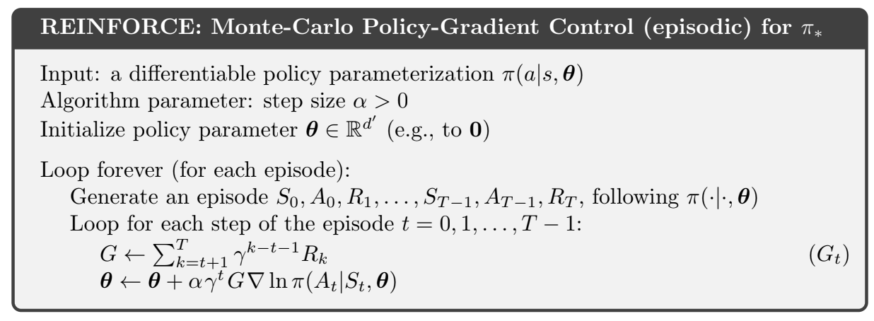
Fig 13.1. REINFORCE Monte Carlo

• good convergence properties (update in the same direction as the performance gradient)
• high variance and slow learning

13.4. REINFORCE with baseline

To reduce variance, the policy gradient theorem can be generalized to include a comparison of the action value to an arbitraty baseline $b(s)$:

$$\nabla J(\theta) \propto \sum_s \mu(s) \sum_a \big(q_{\pi}(s, a) - b(s)\big) \nabla \pi(a|s, \theta) \label{eq:13.11}\tag{13.11}$$

The baseline can be any function as long as it does not vary with $a$:

$$\sum_a b(s) \nabla \pi(a|s, \theta) = b(s) \nabla \sum_a \pi(a|s, \theta) = b(s) \nabla 1 = 0 \label{eq:13.12}\tag{13.12}$$

-> New update rule:

$$\theta_{t+1} \doteq \theta_t + \alpha \big(G_t - b(S_t) \big) \frac{\nabla \pi(A_t| S_t, \theta)}{\pi(A_t|S_t, \theta)} \label{eq:13.13}\tag{13.13}$$

• The baseline can be $0$, so this is a strict generalization of REINFORCE
• Expectation remains unchanged but can help with variance
• In bandits (2.8) the baseline was the average of the rewards seen so far, and it helped a lot with variance
• In MDPs the baseline should vary with the state

One natural choice for the baseline is an estimate of the state value $\hat{v}(S_t, \mathbf{w})$

REINFORCE is a Monte Carlo method for learning the policy parameters $\theta$, so it’s natural to use a Monte Carlo method to learn the state-value weights $\mathbf{w}$

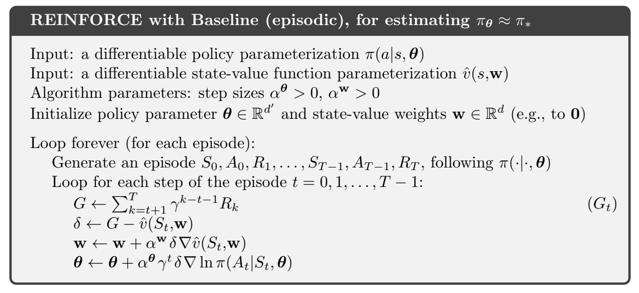
Fig 13.2. REINFORCE with baseline

• We now have two step size parameters $\alpha^{\theta}$ and $\alpha^{\mathbf{w}}$
• For the values ($\alpha^{\mathbf{w}}$) in the linear case it’s “easy”
• It is not very clear for the step size for the policy parameters, whose best value depends on the range of variation of the rewards and on the policy parametrization

13.5. Actor-Critic Methods

• REINFORCE with baseline is not considered an actor-critic method because its state-value function is only used as a baseline, not a critic (aka not used for updating the values of a state with estimates of subsequent states // bootstrapping)
• With bootstrapping we introduce a bias and an asymptotic dependence on the quality of the function approximation
• This bias is often beneficial because it reduces variance

REINFORCE with baseline is unbiased and converge asymptotically to a local minimum but it has a high variance (MC) and thus learns slowly. (+ it’s inconvenient to use online or in continuing setting).

If we use TD methods we can eliminate these inconveniences and with multi-step we control the degree of bootstrapping.

-> For policy-gradient we use actor-critic methods with a bootstrapping critic

13.5.1 One-step actor-critic methods

We start with one-step actor-critic methods without eligibility traces

• fully online and incremental
• simple
• analog to TD(0), Sarsa(0), and Q-learning

How to

1. Replace the full return of REINFORCE by the one-step return
2. Use a learned state-value function as the baseline

$$\begin{align} \theta_{t+1} & \doteq \theta_t + \alpha \big(G_{t:t+1} - \hat{v}(S_t, \mathbf{w}) \big) \frac{\nabla \pi(a| S_t, \theta)}{\pi(a|S_t, \theta)} \label{eq:13.14}\tag{13.14}\\ & = \theta_t + \alpha \big(R_{t+1} + \gamma \hat{v}(S_{t+1}, \mathbf{w}) - \hat{v}(S_t, \mathbf{w}) \big) \frac{\nabla \pi(a| S_t, \theta)}{\pi(a|S_t, \theta)} \label{eq:13.15}\tag{13.15}\\ & = \theta_t + \alpha \delta_t \frac{\nabla \pi(a| S_t, \theta)}{\pi(a|S_t, \theta)} \label{eq:13.16}\tag{13.16} \end{align}$$

The natural state-value function learning method to pair with this is semi-gradient TD(0)

Algorithm

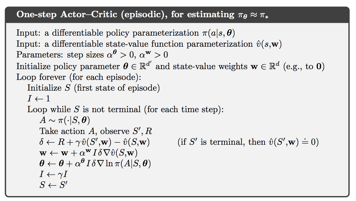
Fig 13.3. One step actor critic

13.5.2. Generalizations

Generalization to n-step methods and then to $\lambda$-return: replace the one-step return by $G_{t:t+n}$ or $G_t^{\lambda}$ respectively

Backward view of the $\lambda$-return algorithm: use eligibility traces for the actor and the critic:

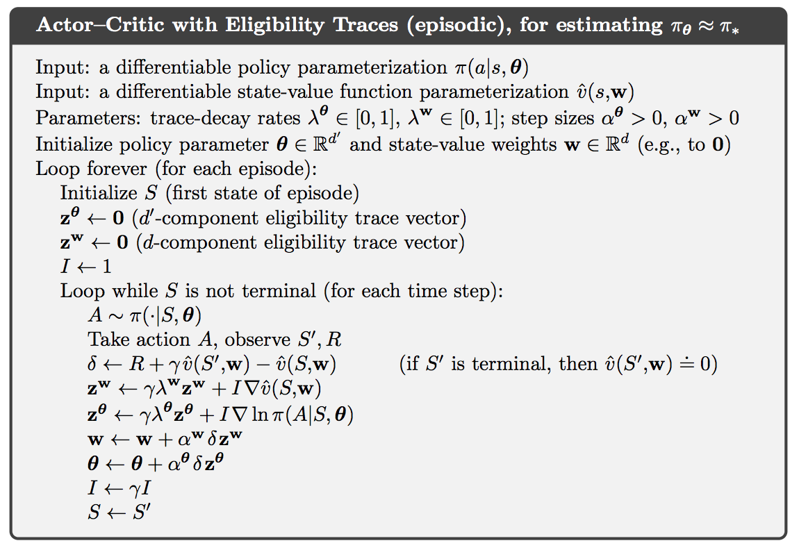
Fig 13.4. Actor critic with eligibility traces

13.6. Policy gradient for continuing problems

From section 10.3 on continuing problems, if we have no episode boundaries we need to define performance in terms of the average rate of reward per time step:

$$\begin{align} J(\theta) \doteq r(\pi) & \doteq \lim_{h \to \infty} \frac{1}{h} \sum_{t=1}^h \mathbb{E}[R_t | A_{0:t-1} \sim \pi] \label{eq:13.17}\tag{13.17}\\ & = \lim_{t \to \infty} \mathbb{E}[R_t | A_{0:t-1} \sim \pi] \label{eq:13.18}\tag{13.18}\\ & = \sum_s \mu(s) \sum_a \pi(a|s) \sum_{s', r} p(s', r | s, a) r \label{eq:13.19}\tag{13.19} \end{align}$$

• $\mu$ is the steady-state distribution under $\pi$, which is assumed to exist and to be independant of $S_0$ [ergodicity assumption]
• $v_{\pi}(s) \doteq \mathbb{E}[G_t|S_t = s]$ and $q_{\pi}(s, a) \doteq \mathbb{E}[G_t|S_t = s, A_t = a]$ are defined with the differential return:

$$G_t \doteq R_{t+1} - r(\pi) + R_{t+2} - r(\pi) + ... \label{eq:13.20}\tag{13.20}$$

With these definitions, the policy gradient theorem remains true for the continuing case (proof in the corresponding section (13.6) of the book).

Algorithm

Fig 13.5. Actor Critic with Eligibility traces in continuing problems

13.7. Policy parametrization for Continuous Actions

Policy gradient methods are interesting for large (and continuous) action spaces because we don’t directly compute learned probabilities for each action. -> We learn statistics of the probability distribution (for example we learn $\mu$ and $\sigma$ for a Gaussian)

Here is the probability density function for the normal distribution for different means and variances:

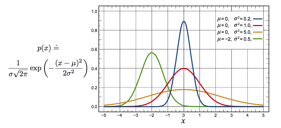
Fig 13.6. Normal distributions for different parameters

To produce a policy parametrization, the policy can be defined as the normal probability density over a real-valued scalar action, with mean and stddev given by parametric function approximators that depend on the state:

$$\pi(a|s, \theta) \doteq \frac{1}{\sigma(s, \theta) \sqrt{2 \pi}} \; \exp\Bigg(- \frac{(a - \mu(s, \theta))^2}{2 \sigma(s, \theta)^2}\Bigg) \label{eq:13.21}\tag{13.21}$$

• $\mu : \mathcal{S} \times \mathbb{R}^{d’} \to \mathbb{R}$ and $\sigma : \mathcal{S} \times \mathbb{R}^{d’} \to \mathbb{R^+}$ are two parametrized function approximators
• Example: the policy’s parameter vector $\theta$ can be divided into two parts:
  • one for the approximation of the mean (linear function)
  • and the other for the stddev (exponential of a linear function):

$$\mu(s, \theta) \doteq \theta_{\mu}^{\top} \mathbf{x}_{\mu}(s) \label{eq:13.22}\tag{13.22}$$ $$\sigma(s, \theta) \doteq \exp\big(\theta_{\sigma}^{\top} \mathbf{x}_{\sigma}(s)\big) \label{eq:13.23}\tag{13.23}$$

• Where the different $\mathbf{x}$’s are state feature vectors
• With these definitions, the methods of this chapter can be used to learn to select real-valued actions

13.8. Summary

• From action-value method to paramztrized policy methods
• actions are taken without consulting action-value estimates
• policy-gradient methods -> update the policy parameter on each step in the direction of an estimate of the gradient of performance

Advantages:

• can learn specific probabilities for taking actions
• can learn appropriate levels of exploration and approach deterministic policies asymptotically
• can handle continuous action spaces
• policy gradient theorem: theoretical advantage

REINFORCE:

• The REINFORCE method follows directly from the policy gradient theorem.
• Adding a state-value function as a baseline reduces variance without introducing bias.
• Using state-value function for bootstrapping introduces bias but is often desirable (TD over MC reasons / reduce variance)
• The state-value function [critic] assigns credit to the policy’s action selections [actor]