Sutton & Barto summary chap 12 - Eligibility Traces
This post is part of the Sutton & Barto summary series.
- 12.1. The lambda return
- 12.2. TD-lambda
- 12.3. n-step truncated lambda-return methods
- 12.4. Redoing updates: The online lambda-return algorithm
- 12.5. True online TD-lambda
- 12.6. Sarsa-lambda
- 12.7 Variable lambda and gamma
- 12.8. Off-policy Eligibility Traces with Control Variates
- 12.9. Watkins’s Q($\lambda$) to Tree-Backup($\lambda$)
- 12.10. Stable off-policy methods with traces
- 12.11. Conclusion
- Eligibility Traces (ET) is a basic mechanism of RL (in TD($\lambda$) the $\lambda$ refers to the use of ET)
- Almost any TD method (Q-learning, Sarsa), can be combined with ET
- It unifies and generalizes Temporal differences (TD) ($\lambda = 0$) and Monte Carlo (MC) ($\lambda = 1$) methods
- ET provides a way to use MC online or in continuing problems
Core of the method:
- we maintain a short term vector $\mathbf{z}_t \in \mathbb{R}^d$ that parallels the long term vector $\mathbf{w}_t$
- when a component of $\mathbf{w}_t$ participates in producing an estimated value, then the corresponding component of $\mathbf{z}_t$ is bumped up and after begins to fade away
- if a non-zero TD occurs before the trace fades away, we have learning (trace-decay $\lambda \in [0, 1]$)
Advantages over $n$-step methods:
- we store a single trace $\mathbf{z}$ rather than the result of $n$ steps in the future
- ET is a backward view instead of a forward view, which is somewhat less complex to implement
12.1. The lambda return
We apply the $n$-step return from chapter 7 to function estimation. The n-step return is the first n rewards + the estimated value of the state reached in n steps, each appropriately discounted:
- A valid update can be done towards any n-step return, but also towards any average of n-step returns
- For example, target could be half the two step return + half the 4 steps return
- Any set can be averaged as long as the weights are positive and sum to 1
- We could average one-step and infinite-step returns to get a way of interrelating TD and MC methods
- Compound update: Update that averages simpler components
The TD($\lambda$) algorithm can be viewed as a particular way of averaging n-step updates, each weighted by $\lambda{(n-1)}$ and normalized by $(1 - \lambda)$ to ensure the weights sum to 1:
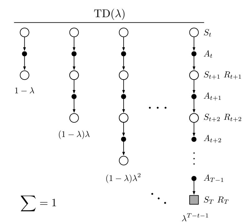
Fig 12.1. Backup diagram for TD($\lambda$). $\lambda = 0$ reduces to the first component only (one-step TD), whereas $\lambda = 1$ gives the full MC update.
The resulting update is towards the lambda return:
Weighting illustration:
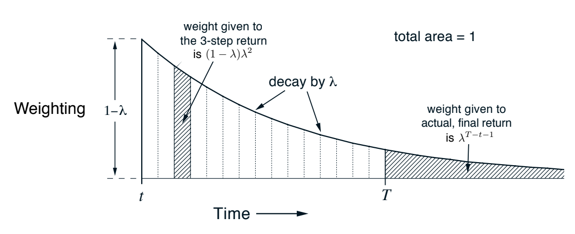
Fig 12.2. Weighting for each of the n-step returns in the $\lambda$-return.
First algorithm based on the lambda-return: offline $\lambda$-return algorithm:
- offline: waits until the end of the episode to make updates
- semi gradient update using the $\lambda$-return as a target
- this is a way of moving smoothly between one-step TD and MC
- theoretical, forward view learning algorithm
Results:
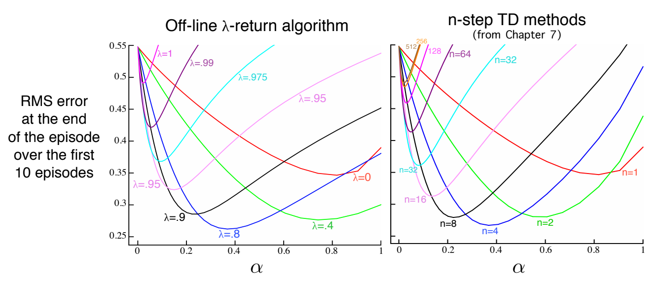
Fig 12.3. Comparison of $\lambda$-return algorithm vs $n$-step TD methods on a 19 states Random Walk example. $\lambda$-return results are slightly better at the best $\alpha$ and $\lambda$ values, and at high $\alpha$.
12.2. TD-lambda
- oldest and most widely used RL algorithms
- first algorithm with a relation between a theoretical forward view and a more practical backward view. The forward view is the “standard” way like n-step, where the update for a state visited at time $t$ depends on the future reward up to $t+n$, which means we have to wait n steps before having enough information to update the “past”. The backward view like ET, maintains the trace vector $\mathbf{z}$ so that the update can be made at the same time.
- TD-lambda approximates the off-line $\lambda$-return algorithm of section 12.1, improving it in 3 ways:
- updates the weight vector at every step and not just at the end of the episode
- computations distributed in time rather than at the end
- can be used in continuing problems
In this section we present the semi-gradient version of TD($\lambda$) with function approximation:
- the eligibility trace $\mathbf{z}$ has the same dimension as $\mathbf{w}$, initialized to $0$
- it is incremented at each time step by the value gradient
- it is decayed at each time step by $\gamma \lambda$
- $\gamma$ is the discount rate
- $\lambda$ is the trace-decay parameter
In linear function approximation, the gradient is just the feature vector $\mathbf{x}_t$ in which case the ET vector is just a sum of past, fading, input vector.
The $\mathbf{z}$ components represent the “eligibility” of each component to learning when a reinforcing event occurs. These reinforcing events are moment-by-moment one-step TD errors:
In TD($\lambda$), the weight vector is updated on each step proportional to the scalar TD error and the vector eligibility trace:
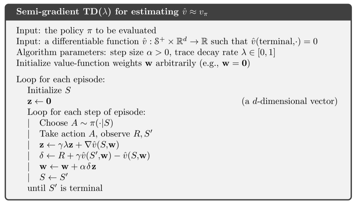
Fig 12.4. Semigradient TD lambda
We have our backward view! At each moment the current TD error is assigned to each prior state according to how much the state contributed to the current ET
- TD(1) can be viewed as a more general MC method. $\lambda = 1$ means that all preceding states are given credit like MC but it can be used in an online continuing setting
- linear-TD($\lambda$) has been proven to converge in the on-policy case if the step-size parameter is reduced over time (see 2.7)
- convergence is not to the minimum-error weight vector but to a nearby weight vector that depends on $\lambda$
12.3. n-step truncated lambda-return methods
- offline $\lambda$-return is limited because we don’t know the $\lambda$-return before the end of the episode
- it is problematic in the continuing case because the $\lambda$-return can depend on an arbitrary large n
- the dependence falls by $\gamma \lambda$ for each step of delay, so maybe we can just truncate it when it’s small enough
- we do this by introducing horizon $h$ which has the same role as time of termination $T$
- in the $\lambda$-return there is a residual weighting given to the true return, here it’s to the longest available n-step return
We use this return in the update:
This can be implemented to start updates at n-1
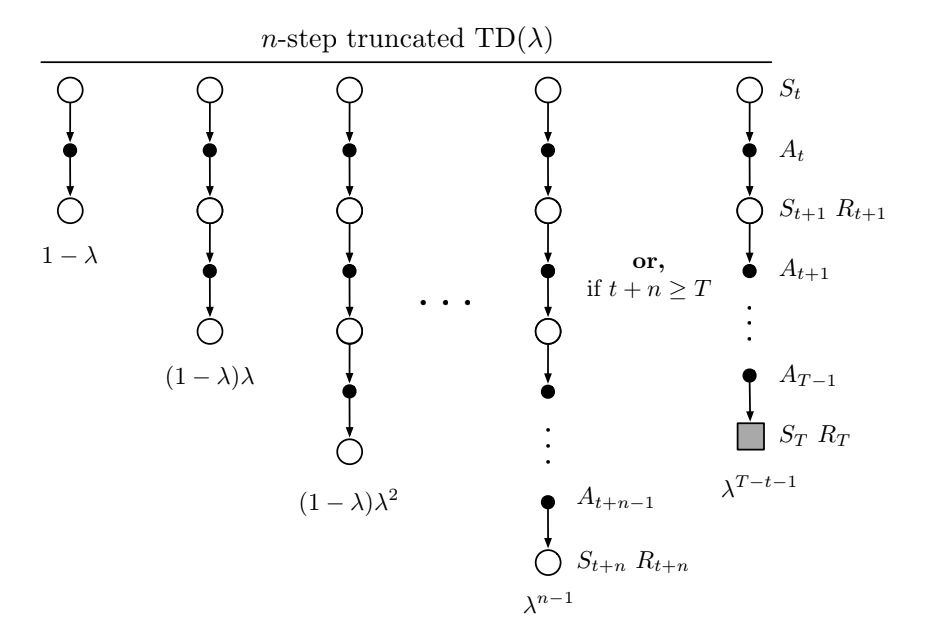
Fig 12.5. Truncated TD
12.4. Redoing updates: The online lambda-return algorithm
- Truncation parameter involves a tradeoff: n should be later to be closer to the true $\lambda$-return, but it should also be sooner to influence behaviour earlier
- This is about getting both (at the cost of computational complexity)
At each time step we go back in time and redo all updates since the beginning of the episode
- the new updates are better because they take the time step’s new data
Convention:
- $\mathbf{w}_0^h$ is the first weight vector in each sequence that is inherited from the previous sequence
- the last weight vector in each sequence $\mathbf{w}_h^h$ defines the ultimate weight-vector sequence of the algorithm
- Example of the first 3 sequences:
General form of the update:
This update, along $\mathbf{w}_t = \mathbf{w}_t^t$ defines the online $\lambda$-return algorithm
12.5. True online TD-lambda
- the algorithm from 12.4 is an ideal that online TD($\lambda$) will try to approximate
- we use ET to invert the forward view to a backward view
- “true” because it’s “truer” to the ideal online $\lambda$-return algorithm than the TD($\lambda$) actually is
The sequence of weight vectors produced by the online $\lambda$-return algorithm can be arranged in a triangle:
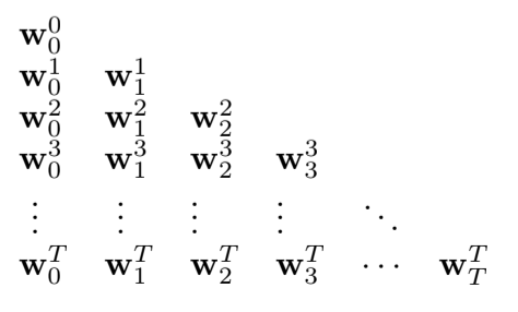
- one row is produced at each time step
- turns out that only the weight vectors in the diagonal are really needed
- first one $\mathbf{w}_0^0$ is the input, last one $\mathbf{w}_T^T$ is the final weight vector, and the intermediate values are used to bootstrap the n-step returns of the updates
- if we can find a way to compute each last vector from the last vector of the previous row, we’re good!
- shorthand $\mathbf{x}_t = \mathbf{x}(S_t)$
- $\delta_t$ is defined as in TD($\lambda$)
- $\mathbf{z}_t$ is the dutch trace defined by:
- proved to produce the same sequence of weights than online $\lambda$-return algorithm
- memory requirements same as TD($\lambda$)
- 50% more computation because there is one more inner-product in the ET update
Algorithm
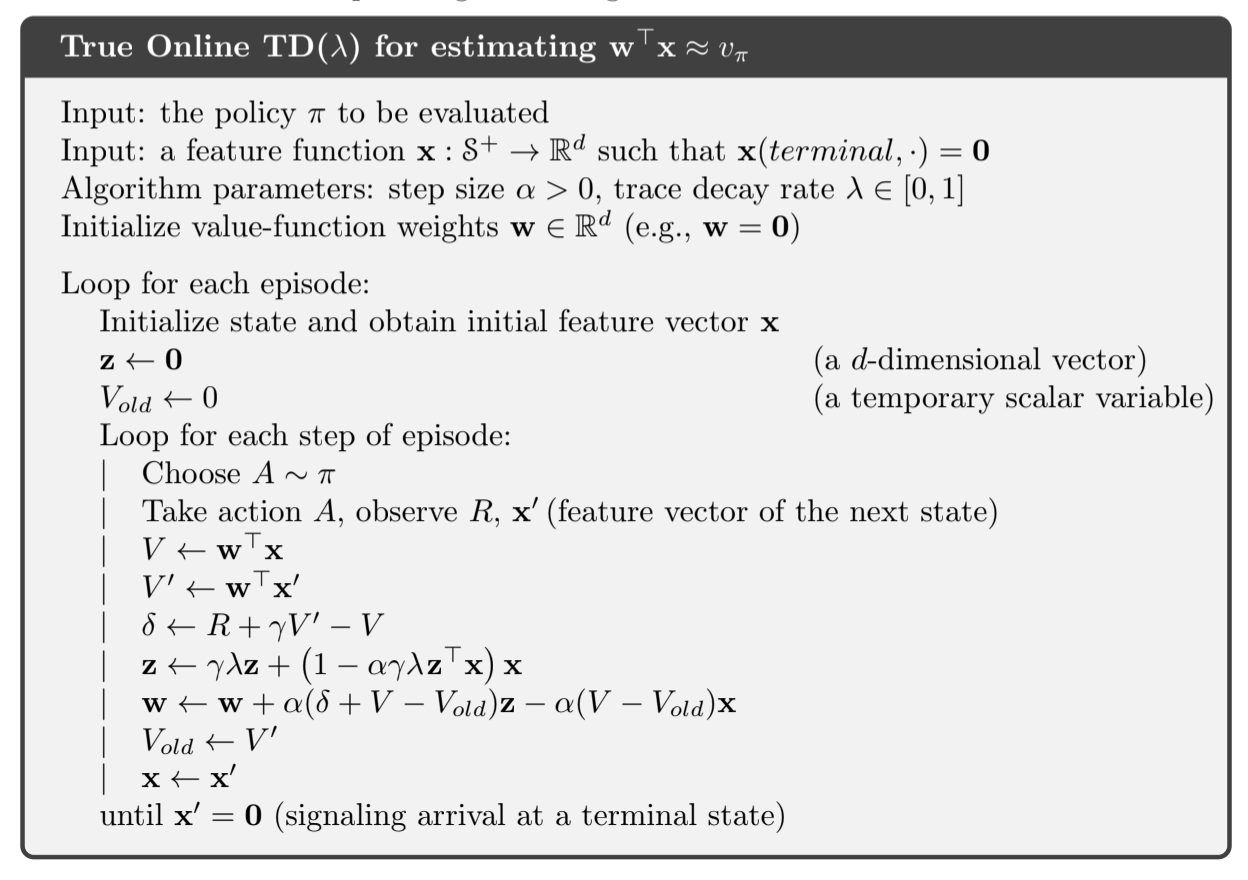
Fig 12.5. True online TD
12.6. Sarsa-lambda
- extend eligibility traces to learn action-values
- to learn approximate values we need to use the action-value form of the n-step return:
- We use this return to form the action-value form of the truncated $\lambda$-return
- $G_t^{\lambda} \doteq G_{t:\infty}^{\lambda}$
- The action-value form of the $\lambda$-return algorithm uses $\hat{q}$ rather than $\hat{v}$:
- This is the forward view. The backup diagram is similar to the TD($\lambda$):
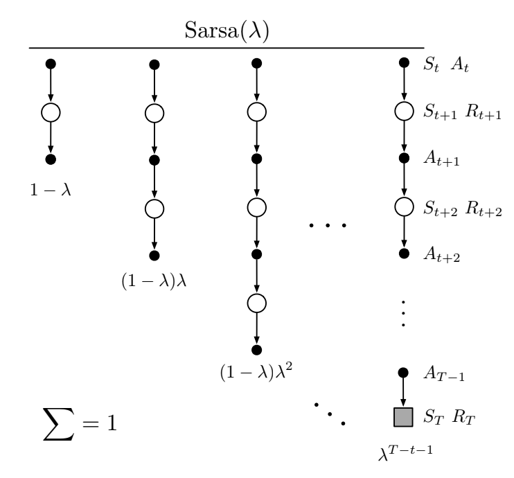
Fig 12.6. Sarsa lambda backup
- first update: one step, second update: 2 steps, final update: complete return
- the weighting on each n-step return is the same as TD($\lambda$)
The backward view of the temporal difference method for action-values, Sarsa($\lambda$), is defined by:
Where the TD error is the action-values one:
Action-value form of the eligibility trace (init to 0):
Pseudocode (using binary features):
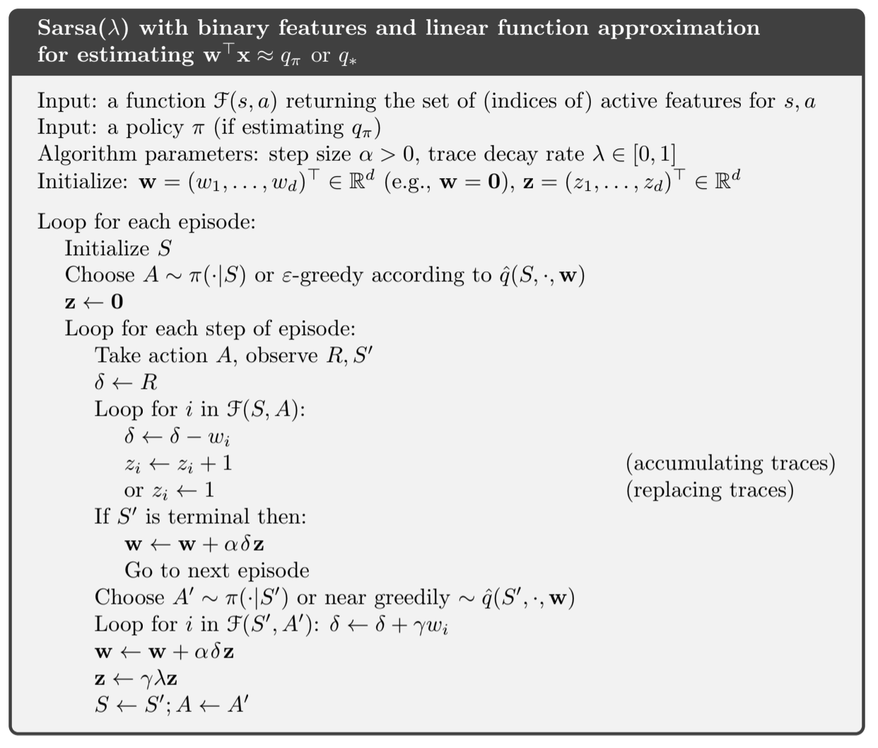
Fig 12.7. Sarsa lambda with binary features
Illustrative example of different methods:
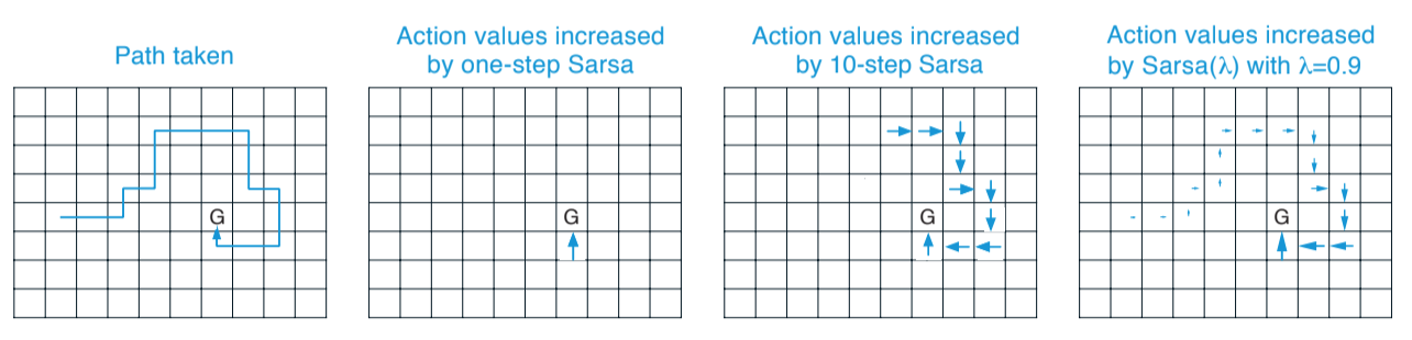
Fig 12.8. Updates made for different methods in a gridworld example. A one-step method would update only the last value, a n-step would update n values, and the use of eligibility traces spread the update using a fading strategy
The Linear function approximation case has an exact $O(d)$ implementation called True Online Sarsa($\lambda$).
12.7 Variable lambda and gamma
- To generalize our TD learning algorithms, we need to generalize the degree of bootstrapping and discounting beyond constant parameters $\lambda$ and $\gamma$
- Now the parameter have a varying value at each time step, $\lambda_t = \lambda(S_t, A_t)$ and $\gamma_t = \gamma(S_t)$
gamma
The function $\gamma$ is a termination function and it now changes the return (the fundamntal Random Variable (RV) whose expectation we seek to estimate)
- to ensure the sums are finite, we require that $\prod_{k=t}^{\infty} \gamma_k = 0$ with probability $1$ for all $t$.
- this definition allows to get rid of episodes, a terminal state just becomes a state with $\gamma = 0$ and which transitions to a start state
lambda
Generalization to variable bootstrapping gives a new state-based $\lambda$-return:
First reward + possibly a second term according to $\gamma_{t+1}$, and that term is
- the estimated value at the state if we’re bootstrapping
- the $\lambda$-return for the next timestep if we are not
Notation:
- s superscript: bootstraps from state-values
- a superscript: bootstraps from action-values
Action-based lambda-return in Sarsa form:
Expected Sarsa form:
where $V$ is generalized to function approximation:
12.8. Off-policy Eligibility Traces with Control Variates
Goal
- We want to incorporate importance sampling with eligibility traces to be able to use off-policy algorithms. To do that, we need:
- To formulate the return
- Use the return in the formulation of the target for the $\mathbf{w}$ update
- Get the eligibility trace $\mathbf{z}$ update
Context
- As a reminder, importance sampling $\rho_t = \frac{\pi(A_t|S_t)}{b(A_t|S_t)}$ is a quantity that is used to weight the return obtained using the behaviour policy, to be abl to learn off-policy
- It often leads to solution that have a high variance, and are slow to converge
- Control variates aims to reduce the variance of the initial estimator (which includes $\rho$), by substracting a baseline that has $0$ expectation.
- Per decision importance sampling with control variates was introduced in section 7.4, and here we develop the bootstrapping version of it:
1: Express return with control variates
In this formulation of the return, the control variate is the $(1 - \rho_t) \hat{v}(S_{t}, \mathbf{w}_{t})$ part, which prevents the return to be $0$ if the experienced trajectory has no chance of occurring under the target policy for example.
2: Approximation of the truncated return
To use this return in a practical algorithm, we will use the truncated version of the return, which can be approximated as the sum of state-based TD errors $\delta_t^s$:
3: Write the forward view update
We can use the truncated return in the forward view update (i.e. without eligibility traces):
4: Eligibility trace update
This update kinda looks like an eligibility-based TD update: the product product would be the ET and it is multiplied by the TD error. But the relationship we’re looking for is an (approximate) equivalence between the forward view update, summed over time, and the backward view update, also summed over time. Let’s start with the forward view update that we sum over time:
- \ref{eq:12.28} uses the summation rule $\sum_{t=x}^y \sum_{k=t}^y = \sum_{k=x}^y \sum_{t=x}^k$
If the entire expression from the second sum left could be written and updated incrementally as an ET, we would have the sum of the backward-view TD update. This is derived in details in the book, but in the end we get the general accumilating trace for state values:
5: Combine everything to get the semi-gradient update
This ET can be combined with the usual semi-gradient parameter update rule for TD($\lambda$) \ref{eq:12.6} to form a general TD($\lambda$) algorithm:
- on-policy $\rho_t$ is always one and we get the usual accumulating trace
- we now have the off-polcy version
-> Extension to the action-values is simplest with Expected Sarsa
At $\lambda = 0$ these algorithms are related to MC, but in a more subtle way since we don’t have any episodes. -> For exact equivalence see PTD($\lambda$) and PQ($\lambda$) [P = provisional]
12.9. Watkins’s Q($\lambda$) to Tree-Backup($\lambda$)
- Extend Q-learning to eligibility traces has been the subject of many methods, Watkins’s is the first one
- Basic principle: decay the ET the usual way as long as a greedy action is taken
- Cut the traces to $0$ when a non-greedy action is taken
Backup diagram:
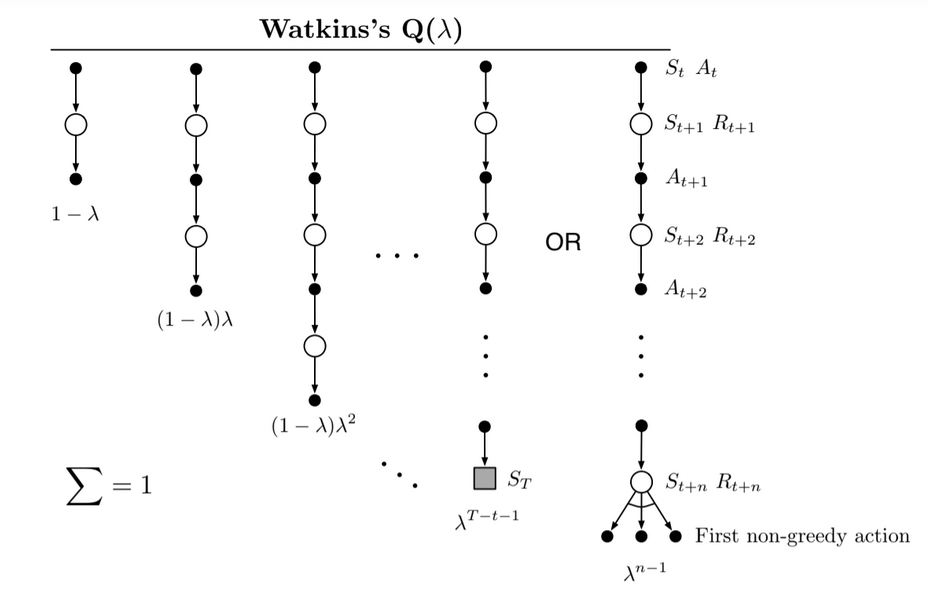
Fig 12.9. Watkins's Q($\lambda$) backup diagram. The series of update ends with the first non-greedy action (or with the end of the episode)
ET with Tree Backups (TB($\lambda$))
- ‘true’ succesor to Q-learning because it has no importance sampling
Backup diagram:
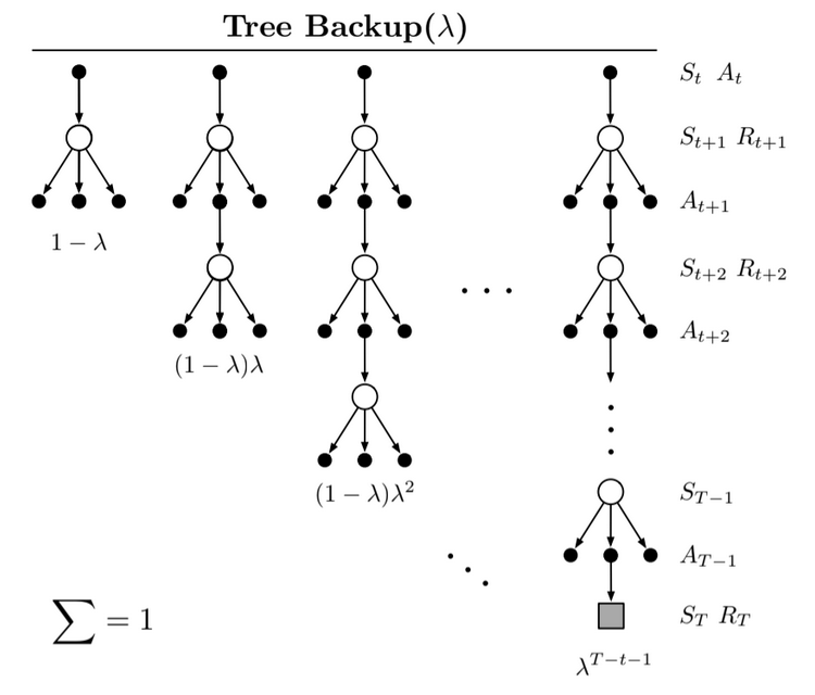
Fig 12.10. Backup diagram for the TB($\lambda$) algorithm
The tree-backup updates are weighted the usual way depending on bootstrapping parameter $\lambda$ For the return we start with the recursive form of the $\lambda$-return using action values, and then expand the bootstrapping case of the target:
Can be written approximately as a sum of TD errors:
Using expectation form of the action-based TD error. Trace update involving target-policy probabilities of the selected actions:
We can combine this to the usual parameter update rule \ref{eq:12.6} to get the TB($\lambda$) algorithm:
12.10. Stable off-policy methods with traces
Here we present 4 of the most important ways. All are based on either Gradient-TD or Emphatic-TD and assume linear function approximation.
GTD($\lambda$)
- analogous to TDC
- our goal is to learn a parameter $\mathbf{w}_{t}$ such that $\hat{v}(s, \mathbf{w}) = \mathbf{w}_t^{\top} \mathbf{x}(s) \approx v_{\pi}(s)$ even from data due to the behaviour policy $b$
with:
- $\mathbf{v}$ is a vector (defined in 11.7) the same size as $\mathbf{w}$
- $\beta$ is a second step-size parameter
GQ($\lambda$)
- Gradient-TD algo for action-values with ET
- Goal: learn $\mathbf{w}_t$ such that $\hat{q}(s, a, \mathbf{w}_t) = \mathbf{w}_t^{\top} \mathbf{x}(s, a) \approx q_{\pi}(s, a)$ from off-policy data
where $\bar{\mathbf{x}}_{t}$ is the average feature vector for $S_t$ under target policy:
$\delta_t^a$ is the expectation form TD error:
The rest is the same as GTD including the update for $v$.
HTD($\lambda$)
- Hybrid state-value algorithm combining GTD($\lambda$) and TD($\lambda$)
- It is a strict generalization of TD($\lambda$) to off-policy, meaning that we find TD($\lambda$) if $\rho_t = 1$
We have:
- a second set of weights $\mathbf{v}$
- a second set of eligibility traces $\mathbf{z}_t^b$ for the behaviour policy
- these $\mathbf{z}_t^b$ reduce to $\mathbf{z}_t$ if $\rho_t$ is 1, causing the last term to be $0$ and algorithm turning TD($\lambda$)
Emphatic TD($\lambda$)
- Extension of Emphatic-TD to eligibility traces
- high variance and potentially slow convergence
- good convergence guarantees and bootstrapping
With:
- $M_t$ emphasis
- $F_t$ followon trace
-
$I_t$ interest (described in 11.8)
- More details in Sutton 2015b
- Details on convergence properties: Yu’s counterexample to see difference with TD($\lambda$) (Ghiassian, Rafiee, and Sutton, 2016).
12.11. Conclusion
- ET with TD errors provide an efficient, incremental way of shiftwing between TD and MC methods
- ET are more general than n-step methods
- MC may have advantages in non-Markov because they do not bootstrap, use ET on TD methods makes them closer to MC and thus more suited to non-Markov cases
- Beware: most of the times we are in a “deadly triad” scenario and we don’t have any convergence guarantee!