Sutton & Barto summary chap 11 - Off-policy methods for approximation
This post is part of the Sutton & Barto summary series.
- 11.1. Semi-gradients methods
- 11.2. Examples of off-policy divergence
- 11.3. Deadly triad of divergence
- 11.4. Linear Value-function Geometry
- 11.5. Gradient Descent in the Bellman Error
- 11.6. The Bellman Error is not learnable
- 11.7. Gradient TD methods
- 11.8. Emphatic TD methods
- 11.9. Reducing the variance
- 11.10. Summary
This chapter is about the extension of off-policy methods from the tabular setting to the approximate setting. It is more painful than the extension of on-policy methods, covered in Chapter 9 and Chapter 10, because we have convergence issues.
Off-policy learning with function approximation poses two main challenges:
- Challenge #1: We need to find the update target
- Challenge #2: The distribution of updates does not match the on-policy distribution.
11.1. Semi-gradients methods
To address challenge #1 and find the update target, we extend methods developped for off-policy to off-policy with approximation using semi-gradient methods.
11.1.1. Semi-gradient reminder
As introduced in Chapter 9.3, semi-gradients arise when it is not possible to compute the true gradient.
We use gradient to update the weight vector $\mathbf{w}$ that is used in approximate methods to produce the values $\hat{v}(S_t, \mathbf{w_t})$. To minimize the error on observed samples, we have a true gradient of the form:
Problem is, we don’t have the true target value $v_{\pi}(S_t)$, so we use an estimate $U_t$:
For methods that don’t bootstrap, such as Monte-Carlo, we can use the return $U_t = G_t$ as the target and our estimate $U_t$ is unbiased, everything is fine and we have convergence guarantees (under certain conditions, of course).
For methods that do bootstrap the estimates $U_t$ for the target value are biased, because they need to use the current values of the weight vector $\mathbf{w}_t$. We then call the method “semi-gradient” since the optimized value ($\mathbf{w}_t$) is also used in the target to compute the gradient.
11.1.2. How semi-gradients will solve challenge #1?
Chapter 7 described off-policy algorithms and we want to convert them to semi-gradient form, to get the full update (challenge #1).
- In the tabular case we update the array ($V$ or $Q$). Now we update a weight vector ($\mathbf{w}$) using the approximate function and its gradient
- Many off-policy algorithms use the per-step importance sampling ratio:
For example, off-policy TD(0) is the same as on-policy TD(0) only with the addition of the $\rho_t$ term:
where $\delta_t$ is defined depending on whether the problem is episodic and discounted or continuous using average reward
For action-values, the one-step algorithm is semi-gradient Expected Sarsa:
with:
Notice that we don’t have importance sampling here!
- In the tabular case it’s normal because Expected Sarsa’s last step is not sampled like Sarsa, it’s a sum over all possible actions, weighted over the target policy, not the behaviour policy so there is no need for importance sampling.
- With function approximation it’s less clear because different $q$ values may contribute to the same approximation, this is an ongoing area of research
- There is importance sampling in the n-step version of Expected Sarsa:
where $G_{t:t+n}$ is defined differently for episodic and continuing case (continuing uses average returns)
- The n-step backup tree algorithm (in Chapter 7) also doesn’t have importance sampling. Here is its semi-gradient:
11.2. Examples of off-policy divergence
This section starts introducing the off-policy challenge #2: the distribution of the updates doesn’t match the on-policy distribution. We have several simple examples that illustrate the issue with off-policy learning, cases where the semi-gradient will diverge.
Example 1
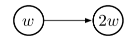
Fig 11.1. First example
- two consecutive states whose estimated value are $w$ and $2w$.
- the parameter vector $\mathbf{w}$ only contains $w$ (this can occur with linear function approximation if the feature vectors are 1 and 2)
- the transition is with probability 1 (importance sampling ratio = 1)
- updates to $w$ will diverge to infinity, since the transition will always look good (leading to a higher value) so the first estimated value will always increase, also making the second estimated value increase (since $w$ is shared). And at every step the system will increase $w$, onwards to infinity.
Example 2
Example 1 was not an entire system, so we seek a complete system that can lead to divergence. One famous system is the Baird’s counterexample:
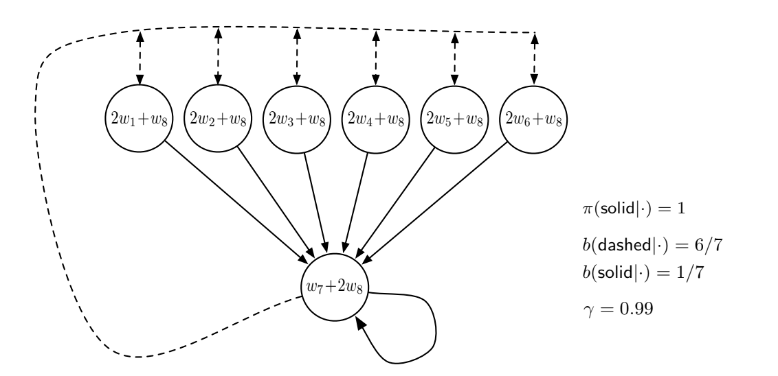
Fig 11.2. Baird's counterexample
In this system, a dashed action leads to one of the six upper states with equal probability, whereas a solid action leads to the seventh state.
- The behavior policy $b$ selects dashed action with probability $\frac{6}{7}$ and solid action with probability $\frac{1}{7}$
- The target policy always takes the solid action
- The reward is always zero
- The discount rate is near 1, $\gamma = 0.99$
- The state-values are estimated under a linear parametrization shown in each state circle (for example, $\mathbf{x}(1) = (2, 0, 0, 0, 0, 0, 0, 1)^{\top}$)
If the reward is always $0$, the true value function is $v_{\pi}(s) = 0$, which can be exactly approximated with $\mathbf{w} = 0$. Since there are $8$ components for the $\mathbf{w}$ vector, there are actually many ways to obtain $0$. This looks easy enough to learn, but if we apply semi-gradient TD(0), the weights actually diverge, no matter how small the step size $\alpha$, as shown in fig 11.3.
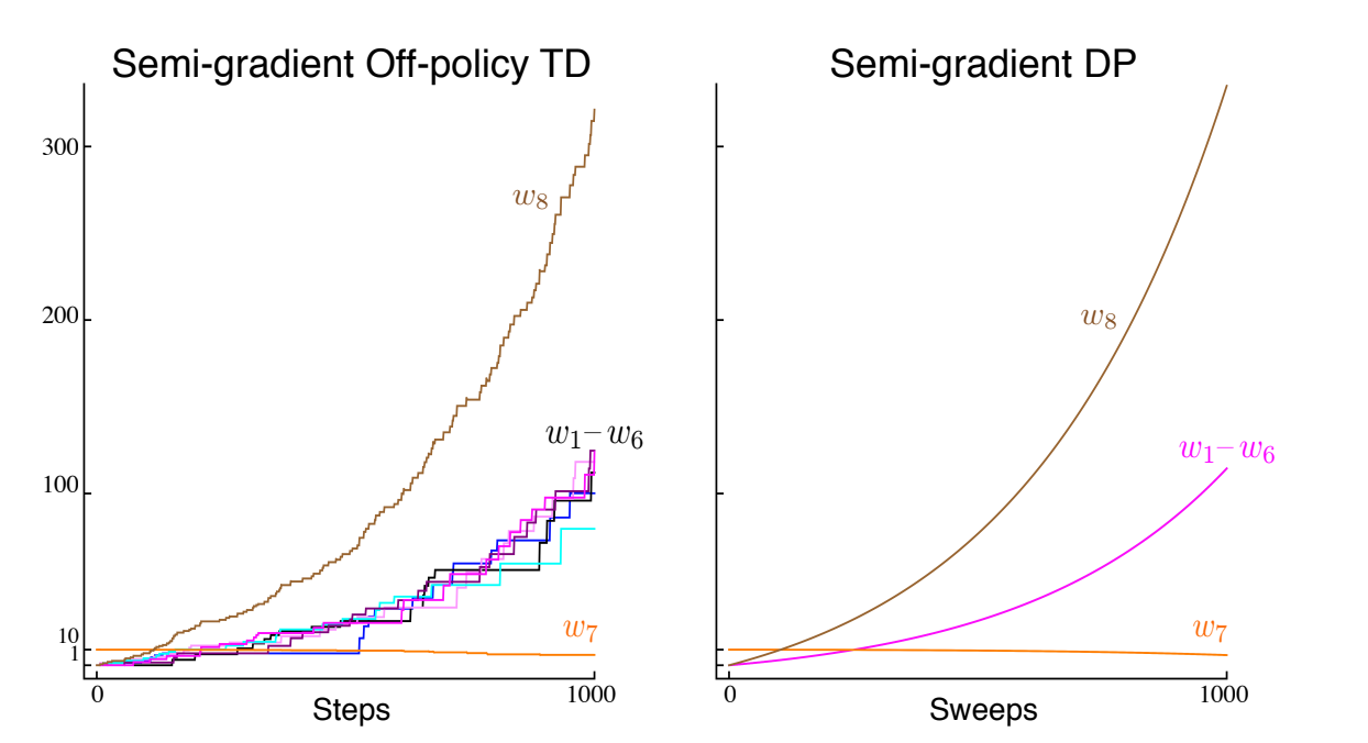
Fig 11.3. Evolution of the components of $\mathbf{w}$ for two semi-gradient algorithms, using $\alpha = 0.01$.
This example, using arguably the simplest bootstrapping method (DP), along with arguably the simplest form of parametrization (linear), show that the combination of bootstrapping and function approximation can be unstable in the off-policy case. A Q-learning version of Baird’s example also exists. For Q-learning though, we can guarantee convergence if the behaviour policy is sufficiently close to the target policy, such as $\varepsilon$-greedy policies.
How to find stability then? The truth is, we don’t really have theoretical guarantees for methods that extrapolate information from observation, such as neural network approximators. We do have stability guarantees for function approximation methods that do not extrapolate, like nearest neighbor averagers, but these methods are not as popular as neural networks.
11.3. Deadly triad of divergence
The instability and risk of divergence arise when we combine three factors:
- function approximation
- bootstrapping: targets that include estimates and are not based only on received rewards (as DP or TD methods)
- off-policy training: distribution different from on-policy (like in DP where the state space sweep is done uniformly)
Instability can be avoided if we remove one of the elements.
- Doing without bootstrapping is possible, but with a loss in computational efficiency (MC!)
- Maybe off-policy is the best to drop (Sarsa instead of Q-learning)
- There is no satisfactory solution because we still need off-policy to do model planning
11.4. Linear Value-function Geometry
In this section we will try to understand better the challenge of off-policy learning by thinking more abstractly about how learning is done with function approximation.
- We have $d$, the number of params in the representation, and $n$ the number of states
- Most states are not representable by our approximation, simply because $d \ll n$
- We can view each representation in a d-dimensional space, and each state in a n-dimensional space
- To make that easier to understand, let’s say we have three states $\mathcal{S} = {s_1, s_2, s_3}$ and two parameters $\mathbf{w} = (w_1, w_2)^{\top}$. A value function $v_{\mathbf{w}}$ is fully defined by its vector $\mathbf{w}$ because it assigns value to each state. Each value function / vector is a point in the 2-dimensional subspace, represented as $v_{\mathbf{w}}$ on figure 11.4.
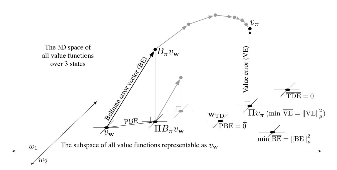
Fig 11.4. Geometry of linear value function approximation
Now we consider a value function for fixed policy $v_{\pi}$. It is too complex to be represented exactly on the $d$-dimensional plane (here $d = 2$), so we need an approximation of it in the 2-dimensional space, so it is represented above. To represent this $v_{\pi}$ in the 2-dimensional plane, we need a projection. So the question is: how do we represent $v_{\pi}$ in the d-dimensional space?. Turns out we have multiple answers to this:
This projection can be made in may ways
- projection operator $\prod$ uses the Value Error norm $\overline{VE}(\mathbf{w}) = || v_{\mathbf{w}} - v_{\pi}||_{\mu}^2$.This solution is found by MC method
- TD methods find other solutions
Bellman error
- The true value function $v_{\pi}$ solves the Bellman equation exactly.
- Approximate methods find approximations $v_{\mathbf{w}}$
- The Bellman error at state $s$ is a measure of the distance between $v_{\pi}$ and $v_{\mathbf{w}}$
- The vector of all Bellman errors for all states is the Bellman error vector $BE$
- The overall size of this vector is the Mean Square Bellman Error $\overline{BE}(\mathbf{w})$
- Interesting methods seek to find the $v_{\mathbf{w}}$ for which $\overline{BE}$ is minimized
Summary
- The Bellman operator $B_{\pi}$ takes the value function out of the d-dimensional subspace and have to be projected back to be followed (PBE)
- $\overline{PBE}$ is the Mean Square Projected Bellman Error
- zero $\overline{PBE}$ = TD fixed point
11.5. Gradient Descent in the Bellman Error
Now that we have a better understanding of the different objectives of value function approximation, we can think about stability in off-policy learning.
- In true SGD, updates are made in the direction of the negative gradient and in expectation go downhill, giving good convergence properties
- Only MC uses true SGD, semi-gradients with bootstraping do not
- To apply SGD we need an objective function, and this section explore objective functions based on the Bellman Error discussed in the previous section
Warning this approach has failed but it’s still interesting to see why
First naive approach
1 Take the minimization of the expected square of the TD error as an objective
2 From the TD error we can compute the Mean Square TD error which looks like this (more detail about the steps of the computation in the book):
3 We can derive the per-step update based on a sample of this expected value:
- This is the same as the semi-gradient TD algorithm \ref{eq:11.4} except for the last term, which completes the gradient and makes a true SGD
- It has excellent convergence properties, however it does not necessarily converge to a desirable place
- Simple examples (like example 11.2 in the book) shows that even for a simple problem, true values can generate larger TD error than other values.
Minimizing TD error is thus naive: by penalizing all TD errors it achieves more like temporal soothing than accurate prediction
Second approach
- Minimize Bellman error instead! (if the exact values are learned, the Bellman error is zero!)
- It gives the residual gradient algorithm, which is biased because $S_{t+1}$ appears in two expectations that are multiplied together
- During interation with the environment only one next state is obtained, so we can’t really sample both expectations at the same time
- Two ways to make it work
- in deterministic environments the next states are necessarily the same so both expectations are correct
- the other way is to obtain two independent samples of the next state (possible in a simulation)
- Good convergence and minimizes the BE
- Still unsatisfactory:
- Slow af
- It seems to converge to the wrong values in function approximation (A-presplit example)
- Third has to do with the BE itself, which is discussed in the next section
11.6. The Bellman Error is not learnable
- It turns out that the Bellman error is not learnable from the observable data. Not learnable in the sense of efficiently learnable in polynomial time, but more in the general sense of leanable at all. So if it’s not learnable from observable data, we’re not going to seek it.
- Example of something not learnable:
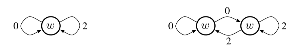
Fig 11.5. Learnability example
- Both Markov Reward Proceses (MRP) output an endless stream of 0 and 2, and it’s impossible to learn that one has one state and the other has two.
- The $\overline{VE}$ introduced in section 9.2 is not learnable but the parameter (the $w$ in fig 11.5) that optimizes for it is! Which makes the $\overline{VE}$ still useful
- If we return to the $\overline{BE}$ (\ref{eq:11.13}), it can be computed from the knowledge of the MDP but not learnable from data, like $\overline{VE}$.
- Unlike $\overline{VE}$ however, its minimum solution is not learnable. (See counterexample 11.4 in the book for more info)
- Other bootstrapping objectives, like $\overline{PBE}$ and $\overline{TDE}$ are learnable from data, and produce solutions different from each other and from $\overline{BE}$
- $\overline{BE}$ is too limited (we need access to the underlying MDP’s dynamics $p$ to compute it) so $\overline{PBE}$ seems a better choice
TL;DR
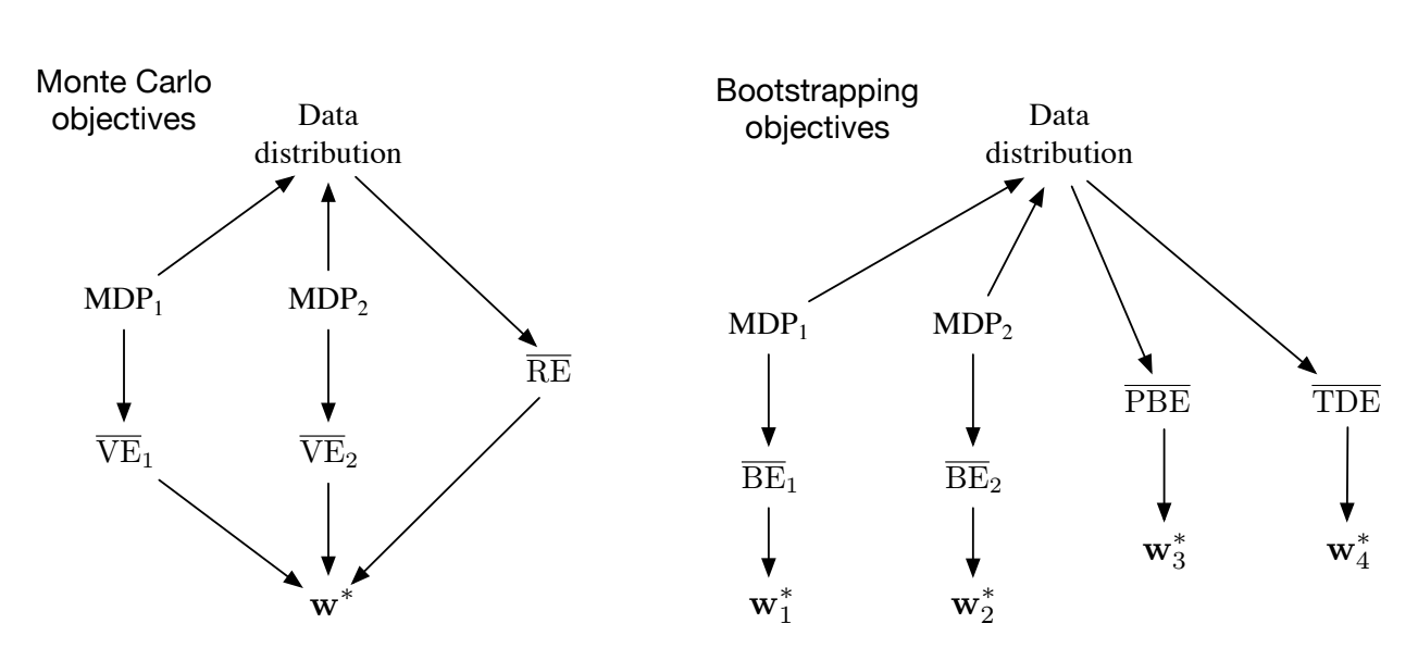
Fig 11.6. Objectives summary
This figure shows the relationship between the data, MDPs, and objectives.
- In the Monte Carlo case, two different MDPs can generate the same data but with different $\overline{VE}$s, proving that the $\overline{VE}$ is not learnable with data alone. But in this case, the optimal parameters $\mathbf{w}^*$ are the same and can also be determined from another objective, the $\overline{RE}$, which is unique for the data distribution.
- For the Bootstraping methods, two MDPs can also produce the same data distribution, their $\overline{BE}$ is different and optimized with different optimal parameters $\mathbf{w}^*$. The $\overline{PBE}$ and $\overline{TDE}$ objectives are learnable from the data distribution.
11.7. Gradient TD methods
- We now consider true Stochastic Gradient Descent (SGD) methods to minimize $\overline{PBE}$ (true SGD -> good convergence)
- In the linear case there is always a solution, the TD fixed point $\mathbf{w}_{TD}$ at which $\overline{PBE}$ is zero (see fig 11.4).
- Least squares method gives a $O(d^2)$ solution, and we seek a $O(d)$ one with SGD
- We still assume linear function approximation
- To derive a SGD method using $\overline{PBE}$, we first need to talk a bit about the projection matrix $\Pi$ that is used to in the definition of $\overline{PBE}$.
Projection matrix
For a linear function approximator, the projection operation is linear, and can be represented by an $|\mathcal{S}| \times |\mathcal{S}|$ matrix:
Where:
- $\mathbf{D}$ denotes the diagonal $|\mathcal{S}| \times |\mathcal{S}|$ with the $\mu(s)$ values on the diagonal ($\mu(s)$ represents how much we care about state $s$, see section 9.2).
- $\mathbf{X}$ denotes the $|\mathcal{S}| \times d$ matrix whose rows are the feature vectors $\mathcal{x}(s)^{\top}$ for each state $s$.
Using these matrices, the squared norm of a vector can be written as:
Objective formulation
Then we can rewrite the $\overline{PBE}$ objective in matrix terms.
Explanation:
- \ref{eq:11.23} is the $\overline{PBE}$ definition (\ref{eq:11.14})
- \ref{eq:11.24} uses \ref{eq:11.22}
- \ref{eq:11.25} uses $\Pi$ definition (\ref{eq:11.21}) and identity $\Pi^{\top} \mathbf{D} \Pi = \mathbf{D} \mathbf{X} (\mathbf{X}^{\top} \mathbf{D} \mathbf{X})^{-1} \mathbf{X}^{\top} \mathbf{D}$
Gradient
The gradient with respect to $\mathbf{w}$ is:
- Turn that into an SGD method: sample something on every timestep that has this quantity on expectation
- If $\mu$ is the distribution of the states visited under the behaviour policy,
- All three factors can be expressed in terms of expectations under this distribution (details for each factors in the book)
End result:
- still the first and last expressions are not independant (same sample vector $\mathbf{x}_{t+1}$) (-> biased)
- we could estimate the 3 factors separately and then combine them but it would be too computationally expensive
- If 2 out of 3 factors are estimated and stored then we sample the last -> still $O(d^2)$
Gradient-TD
- store the product of the two last factors (product of $d \times d$ matrix and $d$ vector so we get a $d$ vector)
- this product is a $d$-vector, like $\mathbf{w}$ itself. We call it $\mathbf{v}$:
- [linear supervised learning] solution to a linear least squares problem that tries to approximate $\rho_t \delta_t$ from experience
- Standard SGD method for finding the $v$ that minimizes the expected squared error is the Least Mean Square (LMS):
- $\beta > 0$ is the step size parameter
- $\rho_t$ importance sampling ratio
- $O(d)$ storage and computation
GTD2
Given $\mathbf{v}$ (\ref{eq:11.30}) we can update our main parameter $\mathbf{w}$ using SGD:
Explanation:
- \ref{eq:11.31} is from the general SGD rule
- \ref{eq:11.32} is using the gradient $\nabla \overline{PBE}(\mathbf{w})$ from \ref{eq:11.28}
- \ref{eq:11.33} is from algebraic arrangements
- The approximation made in \ref{eq:11.34} is using the approximation from \ref{eq:11.29}
- And we remove the expectation to get \ref{eq:11.35} by sampling
This algorithm is called GTD2 and in the last step if the inner product $\mathbf{x}_t^{\top} \mathbf{v}_t$ is done first it is $O(d)$
TD(0) with gradient correction (TDC), or GTD(0)
A better version with more analytic steps between \ref{eq:11.33} and the $\mathbf{v}_t$ substitution gives the following update:
Summary and further reading
- Both GTD2 and TDC involve two learning processes, one for $\mathbf{v}$ and one for $\mathbf{w}$
- asymetrical dependence ($\mathbf{v}$ doesn’t need $\mathbf{w}$ but $\mathbf{w}$ needs $\mathbf{v}$) -> cascade
- usually the secondary learning process ($\mathbf{v}$) is faster
- Extension to non-linear function approximation: Maei et al 2009
- Hybrid TD algorithms
- Gradient-TD combined with proximal methods and control variates -> Mahadevan et al 2014
11.8. Emphatic TD methods
- In this section we explore a major strategy for obtaining a cheap and efficient method for off-policy learning with function approximation
- linear semi-gradient methods are stable under on-policy distribution (9.4)
- it works because there is a match between the on-policy state distribution and the state-transition probabilities under the target policy
- we don’t have this match anymore in off-policy!
Solution: reweight the states, emphasizing some and de-emphasizing others, so as to return the distribution of updates to the on-policy distribution
There is no unique “on-policy distribution”
The one-step Emphatic-TD algorithm for learning episodic state values is defined by:
- $I_t$, the interest, is arbitraty
- $M_t$, the emphasis, is init with $M_{t-1} = 0$
- In Baird’s counterexample, this algorithm converges in theory, but in practice the variance is so high that it’s impossible to use
11.9. Reducing the variance
- off-policy variance > on-policy variance by design
- policy ratios ($\rho$):
- 1 in expected value
- can be as low as 0 in practice
- successive importance sampling ratios are not correlated, so their product is always one
- these ratios multiply the step size in SGD methods so the impact of their variance can be huge
- things that can help:
- momentum
- Polyak-Ruppert averaging
- adaptively setting separate step-sizes for different components of the parameter vector (w)
- weighted importance sampling (chap 5) is well-behaved but still tricky to adapt to function approximation (Mahmood and Sutton 2015)
- off-policy without importance sampling (Munos, Stepleton, Harutyunyan, and Bellemare (2016) and Mahmood, Yu and Sutton (2017))
11.10. Summary
- Tabular Q-learning makes off-policy learning seem easy, as its extensions Expected Sarsa and Tree Backup algorithm
- Extension to function approximation, even linear, is tricky
- SGD in the Bellman Error (BE) doesn’t really work because it’s not learnable
- Gradient-TD methods performs SGD in the projected Bellman error
- Emphatic-TD methods try to reweight updates to be closer to on-policy setting