Sutton & Barto summary chap 05 - Monte Carlo methods
This post is part of the Sutton & Barto summary series.
- 5.1. Monte Carlo Prediction
- 5.2. Monte Carlo methods for Action Values
- 5.3. Monte Carlo control
- 5.4. Monte Carlo control without Exploring Starts
- 5.5. Off-policy Prediction by Importance Sampling
- 5.6. Incremental implementation
- 5.7. Off-policy Monte Carlo Control
- 5.8. Summary
First learning method for estimating value functions and discovering optimal policies. Here we don’t have any knowledge of the environment dynamics, we learn only by experience.
Monte Carlo methods are based on episodes and averaging sample returns. They are incremental in the episode-by-episode sense (not in a step-by-step sense).
As in Dynamic Programming, we adapt the idea of general policy iteration. Instead of computing the value function from our knowledge of the MDP, we learn it from sample returns.
5.1. Monte Carlo Prediction
In this part we focus on learning the state-value function for a given policy.
An obvious way to estimate it from experience is to average the returns observed after visits to that state. As more returns are observed, this value should converge to the expected value.
- We wish to estimate $v_{\pi}(s)$, the value of state $s$ under policy $\pi$
- We have a set of episodes using $\pi$ and passing through $s$
- The first visit of $s$ is the first time $s$ is visited in an episode
- First visit MC method: averages the returns following first visit to $s$
- Every visit MC method: averages the returns after each visit to $s$
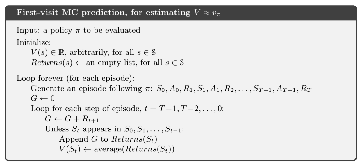 Fig 5.1.First visit
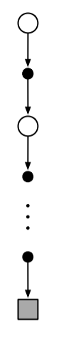
Fig 5.2.Monte Carlo backup diagram
For every-visit version, it’s the same without the check for $S_t$ having occurred earlier in the episode
We can apply backup diagrams to Monte Carlo methods. Contrary to backup diagrams for DP methods, we go all the way to the end of the episode, and we show only the sampled transitions instead of all possible transitions
The estimate for each state in Monte Carlo methods is independent from estimates of other states. In other words, Monte Carlo methods do not bootstrap.
5.2. Monte Carlo methods for Action Values
If the model of a system is not available, it’s better to estimate action values rather than state values. That’s because if we only have the state values we need to do a one-step lookahead that needs the model ($p$ here):
Monte Carlo methods are primarily used to find an estimate of $q_*$, since if we have the q-value we don’t need the model $p$ to find the policy.
Policy evaluation
- every visit MC: estimates the value of $q_{\pi}(s, a)$ as the average of the returns that have followed all the visits to a state-action node
- first visit MC: same but taking only the first time the node has been visited in each episode
Problem: many state-action pairs may not be visited at all (for example if we have a deterministic policy). We must assure continual exploration.
- exploring starts: one way to do it is to start each episode in a state-action pair, each having a non-zero probability of being selected
- Use a stochastic policy with non-zero probability of selecting each action
5.3. Monte Carlo control
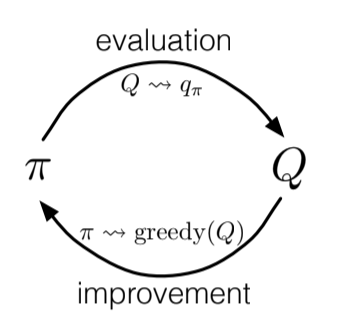
Fig 5.3.Monte Carlo control
This section is about how MC estimation can be used in control (aka approximate optimal policies).
To begin with, we consider the Monte Carlo version of classical policy iteration. We perform alternating complete steps of policy evaluation and policy improvement, beginning with an arbitrary policy $\pi_0$ and ending with the optimal policy and optimal value function.
Policy evaluation: many episodes are experienced, with the approximate action-value function approaching $q_*$ asymptotically. We assume for now that we observe an infinite amount of episodes generated with exploring starts.
Policy improvement is done by making the current policy greedy with respect to the current action-value function.
We construct $\pi_{k+1}$ as the greedy policy with respect to $q_{\pi}(s, a)$. The policy improvement theorem applies to $\pi_{k}$ and $\pi_{k+1}$ because for all $s \in \mathcal{S}$:
This property assures us that each $\pi_{k+1}$ is uniformly better than $\pi_k$ and that in turn ensures that the overall process converges to optimal policy and optimal state-action function.
Assumptions we made
- episodes have exploring starts
- policy evaluation can be done with an infinite number of episodes
To obtain a practical algorithm we will need to remove both assumptions. The second one is easy to remove, since the same issue arises in Dynamic Programming (DP) problems. In both DP and Monte Carlo there are two ways of solving the problem:
- iterate policy evaluation until a threshold of convergence has been reached
- only make a fixed number of steps for policy evaluation (1 in value iteration)
For Monte Carlo methods it’s natural to alternate between evaluation and improvement on a per-episode basis. After each episode, the observed returns are used for policy evaluation, and then the policy is improved at all the states visited during the episode.
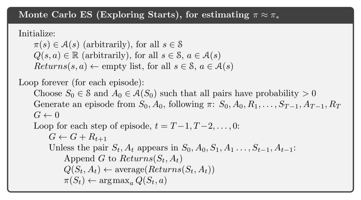
Fig 5.4.Monte Carlo with Exploring starts
All the returns for state-action pairs are averaged, no matter what policy was in force when they were observed. Such a Monte Carlo algorithm cannot converge to any suboptimal policy. If it did, then the value function would eventually converge to the value function for that policy, and that would in turn make the policy change. Stability is achieved only when both policy and value function are optimal. Convergence has not yet been formally proved, see Tsitsiklis, 2012 for a partial solution.
5.4. Monte Carlo control without Exploring Starts
We want to ensure that all actions are selected infinitely often.
- on-policy methods: evaluate and improve the policy that is being used to make decisions (like the Monte Carlo with Exploring Starts method above)
- off-policy methods: evaluate and improve a policy that is different that the one used to generate the data
In this section we focus on the on-policy part and the off-policy will be discussed right after.
On-policy control methods usually use soft policies, meaning that $\pi(s, a) > 0$ for all $a$ and $s$, but gradually shifted closer and closer to a deterministic optimal policy. Here we use an $\varepsilon$-greedy policy, giving $\frac{\varepsilon}{\mid\mathcal{A}(s)\mid}$ to all non-greedy actions and $1 - \varepsilon + \frac{\varepsilon}{\mid\mathcal{A}(s)\mid}$ to the greedy actions.
In plain words, that means that the greedy action is selected most of the time, but sometimes (with probability $\varepsilon$) we select an action at random.
The overall idea of on-policy Monte Carlo control is still that of General Policy Improvement (GPI).
- policy evaluation We use first-visit MC to estimate the action-value for current policy
- policy improvement We can’t just make the policy greedy with respect to the current action-values because it would prevent exploration of non-greedy actions. Fortunately, GPI does not require that the policy be taken all the way to a greedy policy, only that it be moved towards a greedy policy.
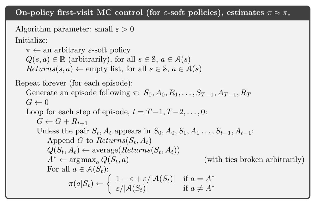
Fig 5.5.On-policy first visit MC
5.5. Off-policy Prediction by Importance Sampling
In the off policy setting, we use two policies:
- the target policy is the policy being learned
- the behavior policy is the policy used to generat behavior
Off-policy methods are usually a bit harder because they require additional notation, and they often have higher variance (the data is from a different policy) and are slower to converge. On the other hand, they are usually more powerful.
We begin the study of off-policy methods by considering the prediction problem, in which both target and behavior policies are fixed. That is we wish to estimate $v_{\pi}$ or $q_{\pi}$ but all we have is a bunch of episodes generated by $b \neq \pi$. We also require that all actions taken by $\pi$ can be taken by $b$, that is $\pi(a |s) > 0$ implies $b(a |s) > 0$ (coverage assumption).
The target policy $\pi$ may be deterministic, often in control it’s the deterministic greedy policy with respect to the current estimate of the value function. This policy becomes a deterministic policy while $b$ remains stochastic and more exploratory. For now in the prediction problem we consider that $\pi$ is given and unchanged.
Importance sampling
Importance sampling is a technique for estimating expected values under one distribution given samples from another, which is exactly what we have! We will weight the returns according to the relative probability of their trajectories occurring under the target and behavior policies, called the importance-sampling ratio.
Given a starting state $S_t$, the probability of subsequent state-action trajectory $A_t, S_{t+1}, A_{t+1}, …, S_T$ under any policy $\pi$ is:
Thus, the importance sampling ratio $\rho_{t:T-1}$ of the trajectory from time step $t$ to $T$ (we stop the ratio at $T-1$ because we don’t have the $A_{T}$ action) is:
The probabilities $p$ that depends on the MDP nicely cancel out and the importance sampling ratio thus depends only on the two policies involved.
Estimating $v_{\pi}$
We still wish to estimate the expected returns under the target policy, but we only have access to the returns $G_t$ of the behavior policy. These returns have the ‘wrong’ expectation $\mathbb{E}[G_t | S_t = s] = v_b(s)$ and cannot be averaged to obtain $v_{\pi}(s)$. This is where the importance sampling ratio comes in:
Now we are ready to give a Monte Carlo algorithm that averages returns from a batch of observed episodes following $b$ to estimate $v_{\pi}(s)$.
notation: if episode $n$ finishes at time step $t = 100$, episode $n+1$ starts at $t = 101$. We can then define $\mathcal{T}(s)$, the set of all time steps in every episode where state $s$ has been visited. For a first-visit method, $\mathcal{T}(s)$ would only include time steps of the first visit to $s$ in each episode.
$T(t)$ denotes the first time of termination after timestep $t$.
$G(t)$ denotes the return after the $t$ to $T(t)$ trajectory.
To estimate $v_{\pi}(s)$ we simply scale the returns by the ratios and average the results:
This is the ordinary importance sampling, because we use a simple average. We can use a weighted average and get the weighted importance sampling:
To understand the difference between the two, consider the estimates after observing a single return.
- for the weighted average, the ratios cancel out and the estimate is equal to the return observed. It’s a reasonable estimate but it’s expectation is $v_b(s)$ rather than $v_{\pi}(s)$ so it’s biased.
- for the ordinary importance sampling, the expectation is $v_{\pi}(s)$ so it’s not biased but it can be a bit extreme. If the trajectory is ten times more likely under $\pi$ than under $b$, the estimate would be ten times the observed return, which would be quite far from the actually observed return.
Infinite variance
More formally we can express the differences between the two estimates (ordinary and weighted) in terms of bias an variance:
- bias the ordinary is not biased but the weighted is.
- variance is generally unbounded for the ordinary estimate because the variance of the ratios can be unbounded whereas in the weighted estimator the largest weight on any single return is one. The weighted estimator has dramatically lower variance in practice and thus is strongly preferred.
Example of variance for ordinary importance sampling when the trajectory may contain loops:
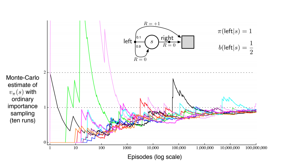
Fig 5.6.Ordinary importance sampling instability
We can verify that the variance of the importance-sampling scaled returns is infinite in this last example. The variance of a random variable $X$ is the expected value of the deviation from its mean $\bar{X}$:
If the mean of the random variable is finite (as in the example), having an infinite variance means that the expectation of the square of the random variable is infinite. Thus, we need only show that the expected square of the importance-sampling scaled return is infinite:
To compute this expectation, we need to break it down into cases based on episode length and termination.
- any episode ending with right action can be ignored because the target policy would never take this action
- We need only consider episodes that involve some number (possibly zero) of left actions that transition back to the nonterminal state, followed by a left action transitioning to termination.
- $G_0$ can be ignored because all considered episodes have a return of 1.
- we need to consider each length of episode, multiplying the probability of the episode’s occurence by the square of its importance-sampling ratio, and add them up:
5.6. Incremental implementation
We want to implement those Monte Carlo prediction methods on a episode-by-episode basis.
To do this, we will take inspiration from chapter 2 (section 2.4) where we incrementally computed Q estimates.
For the on-policy method, the only difference is that here we average returns whereas in chapter 2 we averaged rewards.
For off-policy we need to distinguish between ordinary importance sampling and weighted importance sampling.
In ordinary importance sampling, the returns are scaled by the importance sampling ratio $\rho_{t:T(t)-1}$ (eq \ref{eq:5.4}) then simply averaged like eq \ref{eq:5.6}. For these methods we can again use the incremental methods of chapter 2 but using the scaled returns instead of the reward.
For weighted importance sampling we have to form a weighted average of the returns, and use a slightly different incremental algorithm.
Suppose we have a sequence of returns $G_1, G_2 … G_{n-1}$, all starting in the same state and each with a corresponding random weight $W_i$ (for example $\rho_{t:T(t)-1}$). We wish to form the estimate (for $n \geq 2$):
and keep it up to date as we obtain a single additional return $G_n$. In addition to keeping track of $V_n$, we must maintain for each state the cumulative sum $C_n$ of the weights given to the first $n$ returns. The update rule for $V_n$ ($n \geq 1$) is:
and
A complete algorithm is given below. It extends to the on-policy case (just set $\pi = b$).
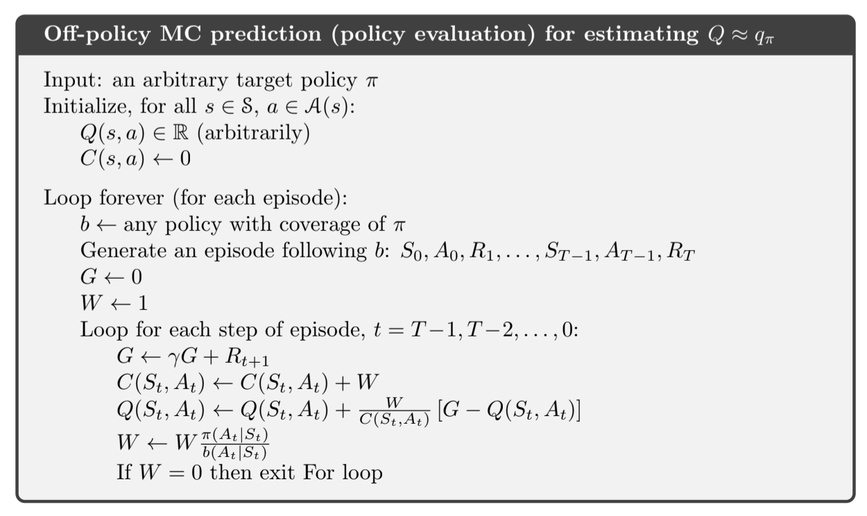
Fig 5.7.Off-policy MC prediction
5.7. Off-policy Monte Carlo Control
In this book we consider two classes of learning control methods:
- on-policy methods: estimate the value of a policy while using it for control
- off-policy methods: these two functions are separated (target vs behavior policies)
Off-policy Monte Carlo control follow the behavior policy while learning about improving the target policy.
The algorithm below shows the off-policy Monte Carlo method based on GPI and importance sampling, for estimating $\pi_*$ and $q_*$.
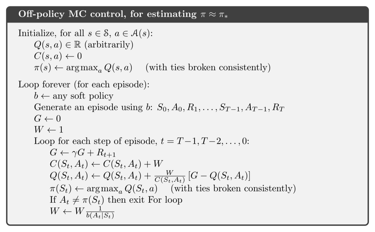
Fig 5.8.Off-policy MC control
A potential problem is that this method only learns from the tails of episodes, when all of the remaining actions are greedy. If nongreedy actions are common, then learning will be slow, particularly for states appearing in early portions of long episodes.
Maybe incorporating TD-learning (next chapter) can help. Also if $\gamma$ is less than one, the idea developped in the next section can help.
5.8. Summary
Monte Carlo methods learn value functions and optimal policies from experience in the form of sample episodes. This has advantages over DP methods:
- We don’t need a model
- We can use simulation or sample models
- It’s easy to focus on a small subset of states
- They don’t update their value estimate for a state based on estimates of successor states (no bootstrapping) thus they can be les harmed by violations of the Markov property
We still use GPI by mixing policy evaluation and policy improvement on an episode-by-episode basis, and for the policy evaluation part we simply average the returns for a given state instead of using the model to compute value for each state.
Exploration is an issue, that we can adress with:
- exploring starts
- off-policy methods
Off-policy methods are based on importance sampling, that weight the return by the ratio of the probabilities of taking the observed action under the two policies, thereby transforming their expectations from the behavior policy to the target policy. Ordinary importance sampling uses a simple average of the weighted returns, whereas weighted importance sampling uses a weighted average.
In the next chapter, we’ll consider methods that make use of experience (like Monte Carlo) but do bootstrap (like DP methods).