Sutton & Barto summary chap 09 - On-policy prediction
This post is part of the Sutton & Barto summary series. This is the first post for the approximate case!
Warning: For this post I’m assuming you are familiar with neural networks and supervised learning so I don’t get into the details.
- About Approximate methods
- Chapter intro
- 9.1. Value-function approximation
- 9.2. The Prediction Objective $\overline{VE}$
- 9.3. Stochastic-gradient and Semi-gradient methods
- 9.4. Linear methods
- 9.5. Feature Construction for Linear Methods
- 9.6. Non-linear function approximation: Neural Networks
- 9.7. Least Squares TD
- 9.8. Memory-Based function approximation
- 9.9. Kernel based function approximation
- 9.10. Looking deeper at on-policy Learning: Interest and emphasis
- 9.11. Summary
About Approximate methods
- Extend tabular methods to problems with arbitrary large state spaces
- In this case, we cannot put every state in a table and just record the associated reward. All our state space don’t fit in memory and even if it did, we don’t have the time to fill our table.
- We are going to use a function approximator that will take the state in input and output the value of the state.
- Generalization issue: we hope that our function approximator will generalize the state space, that is if we get information about one state, it can be useful for similar states too so we can actually learn something for states we didn’t see.
Chapter intro
- Approximating $v_{\pi}$ from experience generated using a known policy $\pi$
- The approximate value function is represented not as a table but as a parametrized function with weight vector $\mathbf{w} \in \mathbb{R}^d$. We hope that $\hat{v}(s, \mathbf{w}) \approx v_{\pi}(s)$
- $\hat{v}$ might be a linear function in features of the state, or a neural network, or the function computed by a decision tree, etc.
- Typically the number of weights is much smaller than the number of states
- Approximation makes RL applicable to partially observable problems. If the parametrized function does not allow the estimated value to depend on certain aspects of the state, then it is just as if those aspects are unobservable.
9.1. Value-function approximation
All the prediction methods covered so far involve an update to an estimated value function that shifts its value towards a backed-up value (update target). Let’s denote an individual update by $s \mapsto v$.
- Monte Carlo (MC):$S_t \mapsto G_t$
- TD(0):$S_t \mapsto R_{t+1} + \gamma \hat{v}(S_{t+1}, \mathbf{w}_t)$
- n-step TD:$S_t \mapsto G_{t:t+n}$
- Dynamic Programming (DP):$s \mapsto \mathbb{E}_{\pi} [R_{t+1} + \gamma \hat{v}(S_{t+1}, \mathbf{w}_t) | S_t = s]$
We can interpret each update as an example of the desired input-output behaviour of the value function.
- up to now the update was trivial: table entry for $s$’s estimated value is shifted a fraction of the way towards the update and other states’ estimates are left unchanged
- now updating $s$ generalizes so that the estimated value of many other states are changed as well
[supervised learning] Function approximation methods expect to receive examples of the desired input-output behaviour of the function they are trying to approximate.
- we view each update as a conventional training example
- it’s important to be able to choose a function approximation method suitable for online learning
9.2. The Prediction Objective $\overline{VE}$
Assumptions we made in the tabular setting:
- No need to specify an explicit objective for the prediction because the learned value could come equal with the true value
- An update at one state does not affect any other state
Now these two are false. Making one state’s estimate more accurate means making others’ less accurate so we need to know which states we care most about with a distribution $\mu(s) \geq 0$ reprensenting how much we care about the error in each state s.
- Error in a state = Mean Squared Error (MSE) between approximate value $\hat{v}(s, \mathbf{w})$ and true value $v_{\pi}(s)$:
On-policy distribution
- Often $\mu$ is chosen to be the fraction of time spent in $s$. Under on-policy training it is called the on-policy distribution
- In continuting tasks, the on-policy distribution is the stationary distribution under $\pi$
In episodic tasks, it depends on how the initial states of episodes are chosen.
- let $h(s)$ denote the probability that an episode begins in each state $s$
- let $\eta(s)$ denote the number of time steps spent, on average, in state $s$ in a single episode
- time is spent in a state $s$ if
- episodes start in $s$
- transitions are made into $s$ from a preceding state $\bar{s}$ in which time is spent
- this system of equations can be solved for the expected number of visits $\eta(s)$. The on-policy distribution is then the fraction of time spent in each state normalized to sum to $1$:
- if there is discounting, we can include $\gamma$ in the second term of the first equation
Performance objective
- $\overline{VE}$ is a good starting point but it’s not clear that it is the right performance objective
- Ultimate goal (reason why we are learning a value function): find a better policy
- If we stick to $\overline{VE}$, the goal is to find a global optimum, a weight vector $\mathbf{w}^*$ for which $\overline{VE}(\mathbf{w}^*) \leq \overline{VE}(\mathbf{w}) \quad \quad \forall \mathbf{w}$.
- Complex approximators may aim for a local optimum
9.3. Stochastic-gradient and Semi-gradient methods
9.3.1. Stochastic gradient
In gradient descent methods,
- the weight vector is a column vector with a fixed number of real valued components, $\mathbf{w} \doteq (w_1, w_2, …, w_d)^T$
- the approximate value function $\hat{v}(s, \mathbf{w})$ is a differentiable function of $\mathbf{w}$ for all $s$
- we update $\mathbf{w}$ at each time step so $\mathbf{w}_t$ is the weight vector at step $t$
- on each step we observe a new example $S_t \mapsto v_{\pi}(S_t)$, assuming for now that we have the true value $v_{\pi}(S_t)$
- we want to find the best possible $\mathbf{w}$, by minimizing error on the observed samples
- $\alpha$ is a positive step-size parameter (learning rate)
- $\nabla f(\mathbf{w})$ denotes the column vector of partial derivatives of the expression with respect to the components of the vector:
- The overall step in $\mathbf{w}_t$ is proportional to the negative gradient of the example’s squared error
- stochastic gradient descent because the update is done on a single example which might have been selected stochastically
- over many examples we make many small steps and the overall effect is to minimize an average performance measure (here $\overline{VE}$)
- convergence to a local optimum is guaranteed depending on $\alpha$
9.3.2. True value estimates
- What about when we don’t know the true value $v_{\pi}(S_t)$ but only have an approximation $U_t$? Just plug it in place of $v_{\pi}(S_t)$ in the update:
9.3.2.1. Monte Carlo
- If $U_t$ is an unbiased estimate (like MC), then we have convergence guarantees under certain conditions for $\alpha$
- $U_t = G_t$
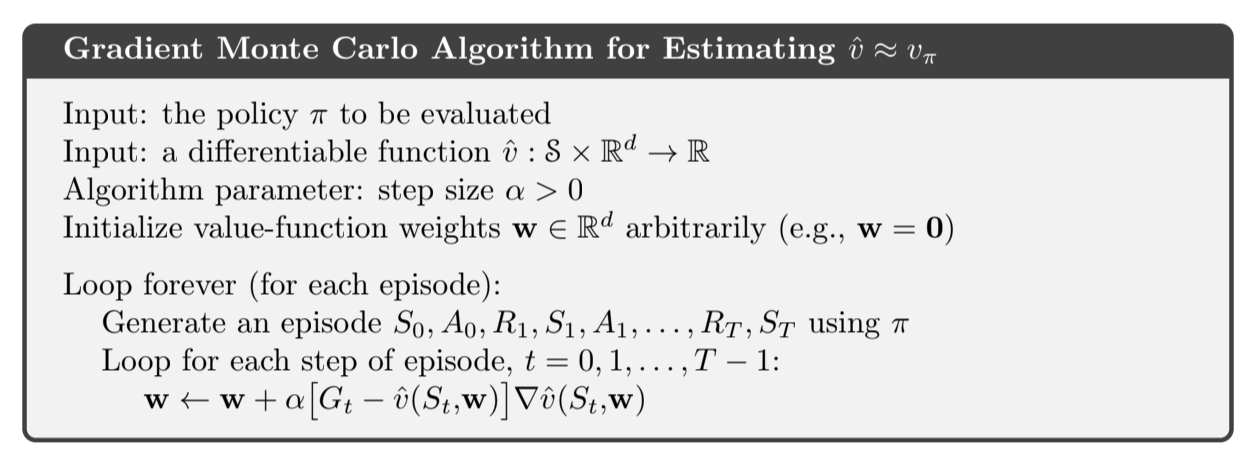
Fig 9.1. Gradient Monte Carlo
9.3.2.2. Bootstrapping
- $U_t = G_{t:t+n}$ (n-step)
- $U_t = \sum_{a, s’, r} \pi(a|S_t) p(s’, r|s, a)[r + \gamma \hat{v}(s’, \mathbf{w}_t)]$ (DP)
- All biased estimates because they use the current value of the weight vector $\mathbf{w}_t$
- semi-gradient methods, they do not converge as robustly as gradient methods but do converge reliably in important cases like linear case discussed after
- enable fast learning with online setting
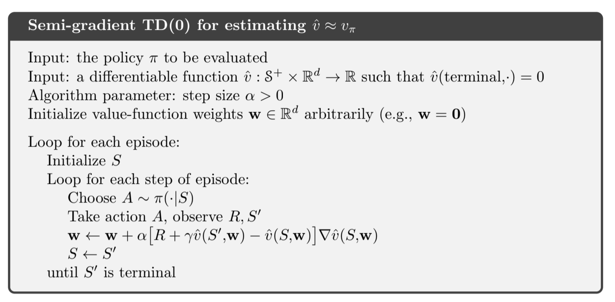
Fig 9.2. Gradient TD
9.3.2.3. State Aggregation
Simple form of generalizing function approximation in which states are grouped together with one estimated value (one component of $\mathbf{w}$) per group.
9.4. Linear methods
One of the simplest cases for function approximation is when the approximate function $\hat{v}(\cdot, \mathbf{w})$ is a linear combination of the weight vector $\mathbf{w}$. In this setting, every state is represented as a vector $\mathbf{x}(s)$ the same length as $\mathbf{w}$ and the approximated state-value is just the inner product between $\mathbf{w}$ and $\mathbf{x}(s)$:
- $\mathbf{w}$ is the weight vector
- $\mathbf{x}(s)$ is a feature vector representing state $s$
- For linear methods, features are basis functions because they form a linear basis of the set of approximate functions
- Using Stochastic Gradient Descent (SGD) with linear function approximation is easy because the gradient of the approximate value function with respect to $\mathbf{w}$ is:
- Thus the linear case SGD update is:
- Easy form that has only one optimum so any method that is guaranteed to converge to or near a local optima is guaranteed to converge to or near a global one.
9.4.1. Semi-gradient convergence
- Semi-gradient TD(0) also converges to a point near the local optimum under linear function approximation
- Notation: $\mathbf{x}_t = \mathbf{x}(S_t)$ shorthand
Once the system has reached steady state, for any given $\mathbf{w}_t$ the expected next weight vector can be written:
where:
- $\mathbf{b} \doteq \mathbb{E}[R_{t+1} \mathbf{x}_t] \in \mathbb{R}^d$
- $\mathbf{A} \doteq \mathbb{E} \big[ \mathbf{x}_t(\mathbf{x}_t - \gamma \mathbf{x}_{t+1})^T\big] \in \mathbb{R}^d \times \mathbb{R}^d$
From $\mathbb{E}[\mathbf{w}_{t+}|\mathbf{w}_t] = \mathbf{w}_t + \alpha(\mathbf{b} - \mathbf{A} \mathbf{w}_t)$, it is clear that, if the system converges, it must converge to the weight vector $\mathbf{w}_{TD}$ at which:
This quantity $\mathbf{w}_{TD}$ is called the TD fixed point and the semi-gradient TD(0) converges to this point
- $A$ needs to be positive definite to ensure that $A^{-1}$ exists and to ensure stability (shrinking of $\mathbf{w}$)
Expansion bound
At the TD fixed point, it has also been proven that $\overline{VE}$ is within a bounded expansion of the lowest possible error (attained by the Monte Carlo method)
- $\gamma$ is often near 1 so the expansion factor can be large
- but TD method have much lower variance than MC and are faster
- an analogous bound can be found for other on-policy bootstraping methods (for example DP)
- one-step action-value methods such as semi-gradient Sarsa(0) converge to an analogous fixed point and bound
- for episodic tasks there is also a bound (Bertsekas and Tsitsiklis 1996)
Pseudocode
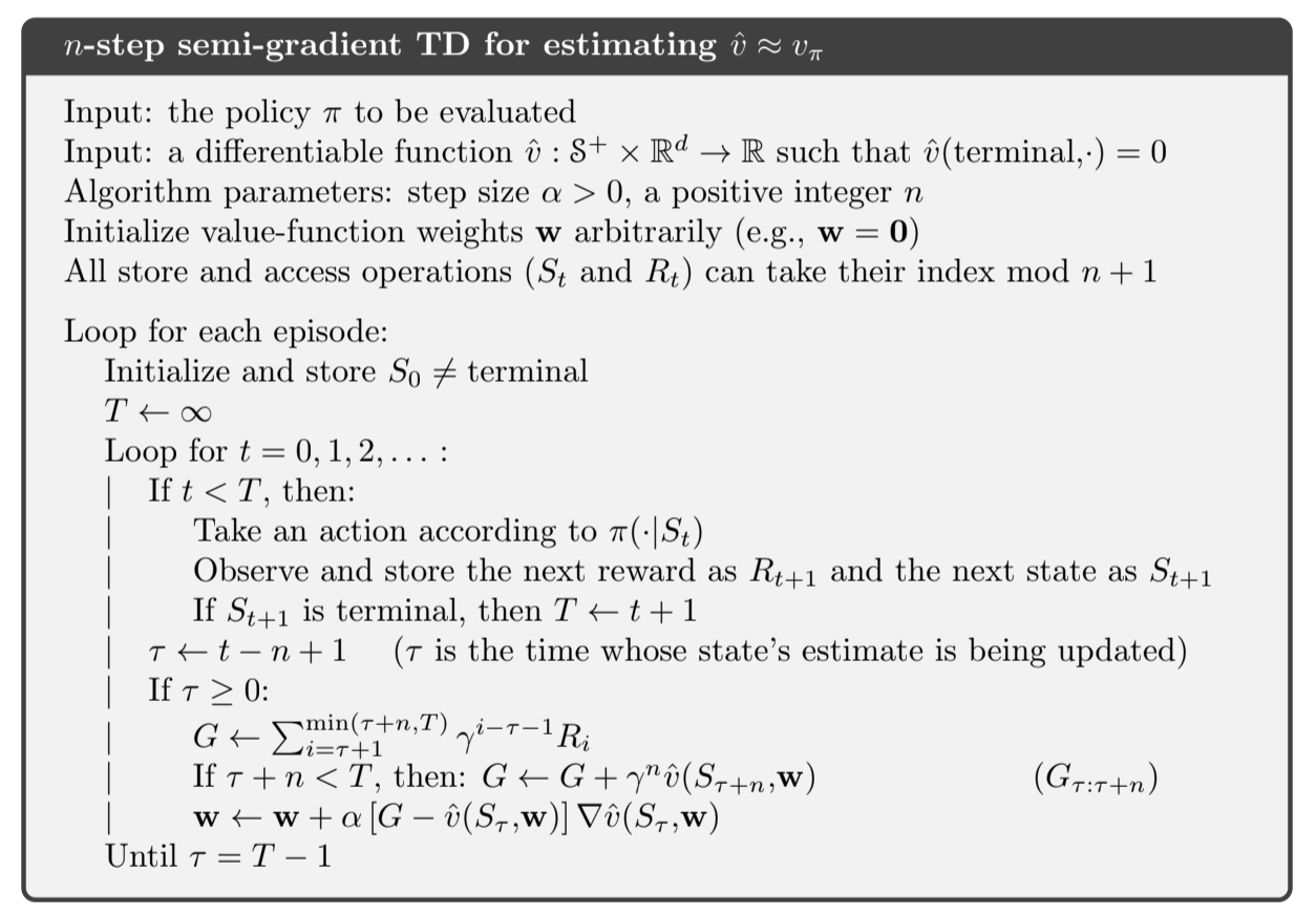
Fig 9.3. $n$-step semi gradient
The key equation of this algorithm is:
where the n-step return is generalized to:
9.5. Feature Construction for Linear Methods
One part of function approximation is that states are represented by feature vectors. Here are several ways to represent the states:
9.5.1. Polynomials
For example a state has two numerical dimensions, $s_1$ and $s_2$. $\mathbf{x}(s) = (s_1, s_2)^T$ is not able to represent any interaction between the two dimensions, so we can represent s by: $\mathbf{x}(s) = (1, s_1, s_2, s_1 s_2)^T$. The initial 1 feature allows for the representation of affine functions in the original state numbers.
It is generally necessary to select a subset of the feature for function approximation. This can be done using prior beliefs about the nature of the functions to be approximated.
9.5.2. Coarse coding
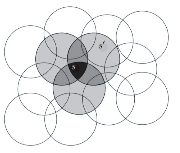
Fig 9.4. Coarse coding. generalization between two states depend on the number of circles in common
- features are circles in the 2D space
- assuming linear gradient descent function approximation, each circle has a corresponding weight (an element of $\mathbf{w}$) that is affected by learning.
- if we train at one state, the weights of all circles of that state will be affected and it will thus affect all states in the union of those circles
9.5.3. Tile coding
- Coarse coding for multi-dimensional continuous spaces
- Receptive fields of the features are grouped into partitions of the state space (each partition is called a tiling and each element of the partition is a tile)
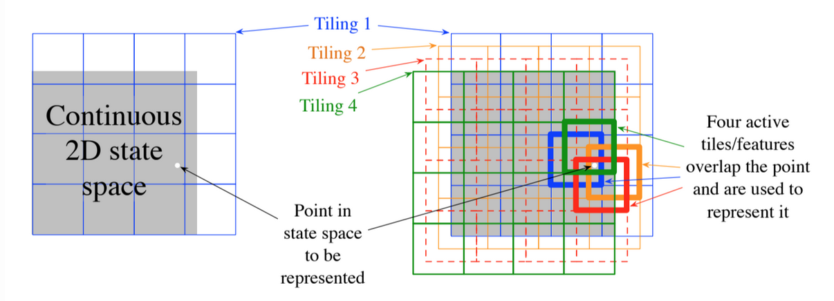
Fig 9.5. Tile coding. Overlapping grid tilings offset from one another by a uniform amount
9.5.4. Radial Basis Function (RBF)
- Generalization of coarse coding to continuous-valued features (instead of a feature being 0 or 1, it can be anything in the interval)
- A typical RBF feature $x_i$ has a Gaussian response dependent only on the distance between the state and the feature’s prototypical or center state $c_i$, and relative to the feature’s width $\sigma_i$:
- The norm or distance metric can be chosen in the most appropriate way. One-dimensional example with Euclidean distance metric:
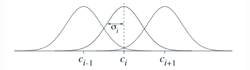
Fig 9.6. One dimensional radial basis function
- Advantage: they produce approximate functions that vary smoothly and are differentiable
- Doubts on practival significance
- An RBF network is a linear function approximator using RBFs for its features.
- Some learning methods for RBF networks change the center and widths of the features as well, making them nonlinear function approximators
- Nonlinear methods may be able to fit target functions much more precisely [greater computational complexity]
9.6. Non-linear function approximation: Neural Networks
In RL, neural networks can use TD errors to estimate value functions, or they can aim to maximize expected reward as in gradient bandit or a policy-gradient algorithm (as we will see in chapter 13).
9.7. Least Squares TD
-> Direct computation of the TD fixed point instead of the iterative method
Recall that TD(0) with linear function approximation converges asymptotically to the TD fixed point:
- $\mathbf{b} \doteq \mathbb{E}[R_{t+1} \mathbf{x}_t]$
- $\mathbf{A} \doteq \mathbb{E} \big[ \mathbf{x}_t(\mathbf{x}_t - \gamma \mathbf{x}_{t+1})^T\big]$
The Least Squares TD Algorithm (LSTD) computes directly estimates for $\mathbf{A}$ and $\mathbf{b}$:
- $\hat{\mathbf{b}}_t \doteq \sum_{k=0}^{t-1} R_{t+1} \mathbf{x}_k$
- $\hat{\mathbf{A}}_t \doteq \sum_{k=0}{t-1} \mathbf{x}_k(\mathbf{x}_k - \gamma \mathbf{x}_{k+1})^T + \varepsilon \mathbf{I}$
where:
- $\mathbf{I}$ is the identity matrix
- $\varepsilon \mathbf{I}$ ensures that $\hat{\mathbf{A}}$ is always invertible
It seems that these estimates should be divided $t - 1$ and they should, but we don’t care because when we use them we effectively divide one by another.
LSTD estimates the fixed point as:
Complexity
- The computation involves the inverse of A, so complexity $O(d^3)$
- Fortunately our matrix has a special form of the sum of outer products, so the inverse can be computed incrementally with only $O(d^2)$. This is using the Sherman-Morrisson formula
- Still less efficient than the $O(d)$ of incremental version, but can be handy depending on how large d is.
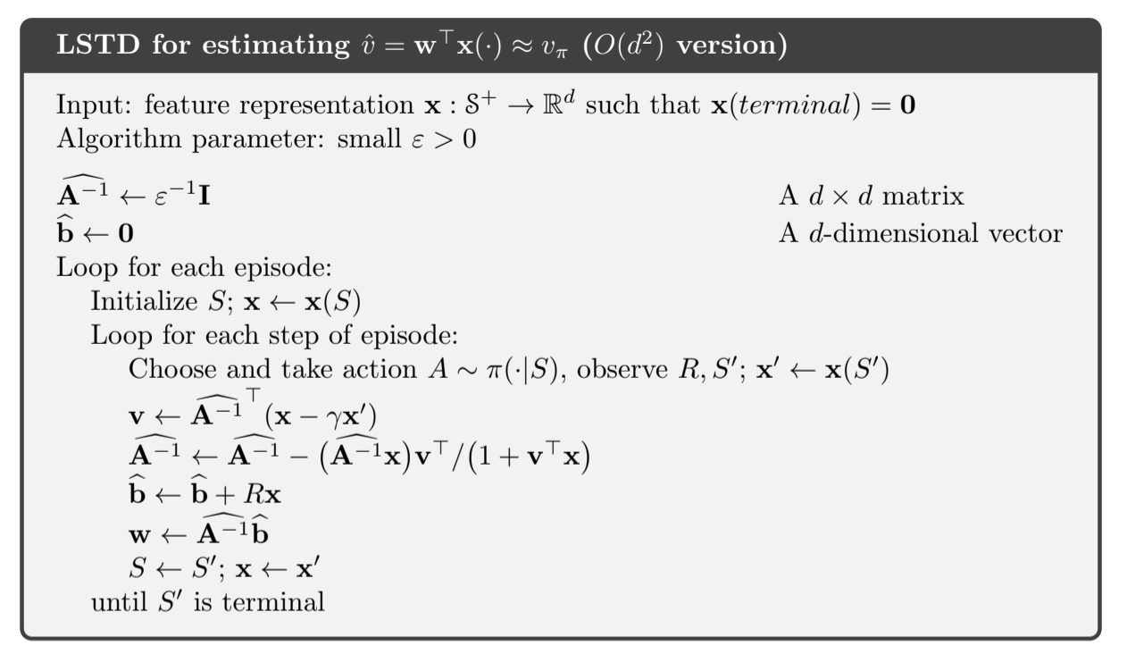
Fig 9.7. LSTD
9.8. Memory-Based function approximation
So far we discussed the parametric approach to function approximation. The training examples are seen, used by the algorithm to update the parameters, and then discarded.
Memory-based function approximation saves the training examples as they arrive (or at least a subset of them) without updating the parameters. Then, whenever a value estimate is needed, a set of examples is recovered from memory and used to produce a value estimate for the queried state.
There are many different memory-based methods, here we focus on local learning:
- approximate a function only in the neighborhood of the current query state
- retrieve states in memory based on some distance measure
- the local approximation is discarded after use
Some examples:
- nearest neighbor method: local example where we retrieve from memory only the closest state and return that state’s value as an approximation
- weighted average: retrieve a set of closest states and weight their value according to the distance
- locally weighted regression: similar but fits a surface to the values of the nearest states with a parametric approximation method
Properties of non-parametric memory methods:
- no limit of functional form
- more data = more accuracy
- experience effect more immediate to neighboring states
- retrieving neighoring states can be long if there are many data in memory (use of k-d trees may improve speed)
9.9. Kernel based function approximation
Memory-based methods depend on assigning weights to examples $s’ \mapsto g$ depending on the distance between the query state $s$ and $s’$. The function that assign weights is called a kernel function or simply a kernel. $k(s, s’)$ can be viewed as a measure of the strength of the generalization between $s$ and $s’$.
Kernel regression is the memory-based method that computes a kernel weighted average of all examples stored in memory:
where:
- $\hat{v}$ is the return value approximation for query state $s$
- $\mathcal{D}$ is the set of stored examples
- $g(s’)$ denotes the target value for a stored state $s’$
A common kernel is the Gaussian radial basis function (RBF) used in RBF function approximation. RBFs are features whose centers can be either fixed at the beginning or ajusted during learning. For the fixed version, it’s a linear parametric method whose parameters are the weights of each RBF, typically learned with SGD. Approximation is a form of linear combination of the RBFs.
Kernel regression with RBF differs a bit:
- memory-based: the RBFs are centered on the states of stored examples.
- nonparametric: no parameters to learn
In practice, the kernel is often the inner product:
9.10. Looking deeper at on-policy Learning: Interest and emphasis
- in this chapter we treated all the states as if they were equally important
- we often have more interest in some states or some actions
The on-policy distribution is defined as the distribution of states encountered in the MDP while following the target policy. Generalization: Rather than having one policy for the MDP, we will have many. All of them are a distribution of states encountered in trajectories using the target policy, but they vary in how the trajectories are initiated.
New concepts:
- New random variable $I_t$, called interest, indicating the degree to which we are interested in accurately valuing a state (or state-action pair) at time $t$. The $\mu$ in the prediction objective is now defined as the distribution of states encountered while following the target policy, weighted by interest.
- Another new random variable $M_t$, called emphasis. This non-negative scalar multiplies the learning update and thus emphasizes or de-emphasizes the learning done at time $t$.
Emphasis is determined recursively from the interest:
- $0 \leq t < T$
- $M_t \doteq 0$ for all $t < 0$
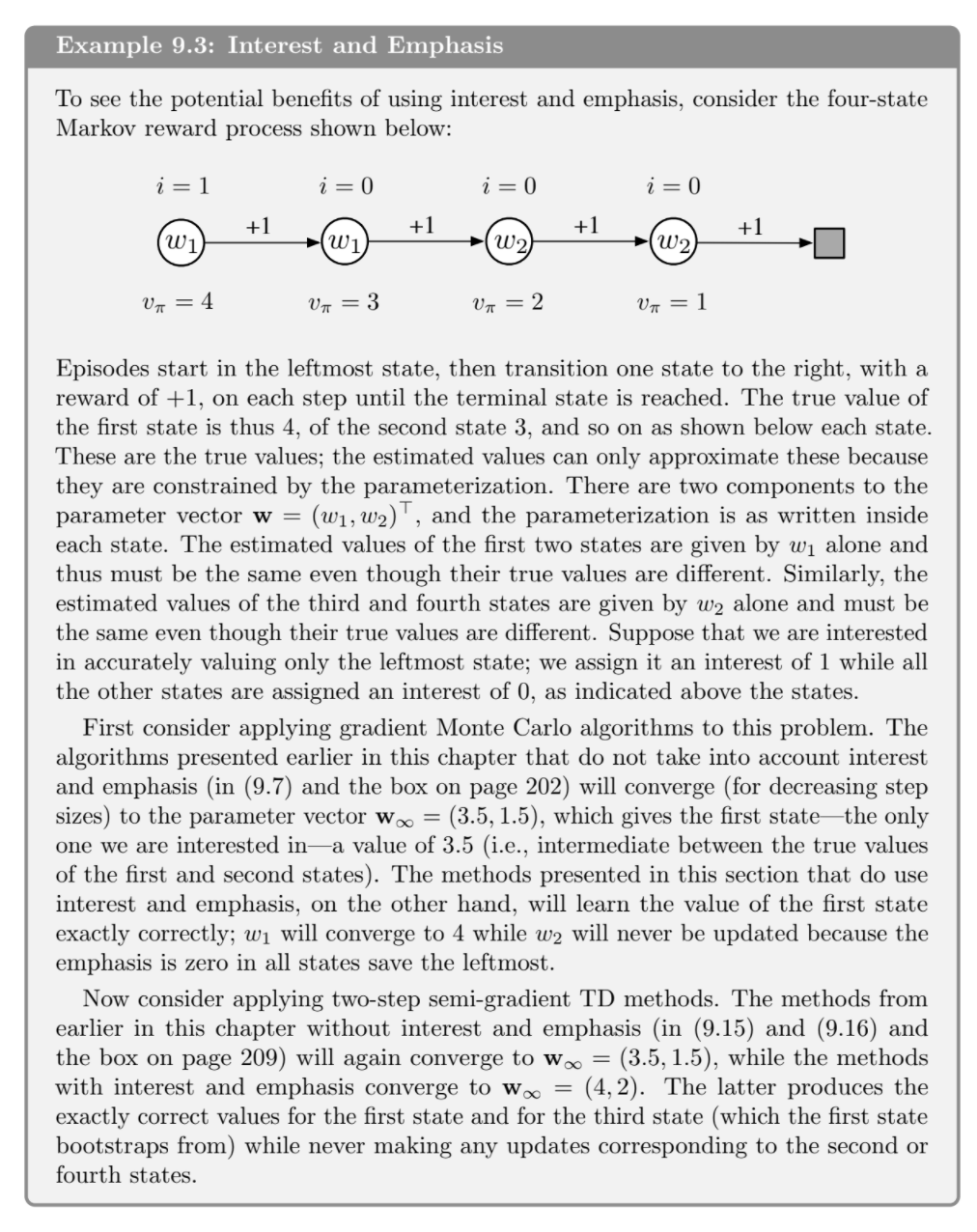
Fig 9.8. Example
9.11. Summary
- we need generalization and supervised learning function approximation can do that, by treating each update as a training example
- crucial use of a weight vector $\mathbf{w}$ as the parameters in parametrized function approximation
- the $\overline{VE}$ measures gives an error to rank the different approximations
- use SGD to find a good weight vector, also semi-gradients methods like TD methods where bootstrapping makes the weight vector appear in the update target
- good results for semi-gradient methods in the linear case which is the most well understood theoretically
- LSTD to find a solution analytically when the number of weights is reasonable
- nonlinear methods -> deep reinforcement learning