Sutton & Barto summary chap 04 - Dynamic Programming

This post is part of the Sutton & Barto summary series.

• 4.1. Policy Evaluation (prediction)
  • Implementation details
• 4.2. Policy Improvement
  • Policy improvement theorem
  • Proof
  • Policy improvement
• 4.3. Policy iteration
  • Implementation
  • Policy iteration for action values
• 4.4. Value Iteration
  • Optimal policy (to build intuition about why value iteration works)
  • Value Iteration
• 4.5. Asynchronous Dynamic Programming
• 4.6. Generalized Policy Iteration
• 4.7. Efficiency of Dynamic Programming
• 4.8. Summary

Dynamic Programming (DP) refers to a collection of algorithms that can be used to compute the optimal policies given a perfect MDP. The assumptions are strong, but DP provides a firm foundation for other methods.

The key idea in DP is the use of the value functions to organize the search for good policies.

• dynamic: sequential or temporal component to the problem
• programming: optimising a “program”, i.e. a policy

Dynamic programming is a method for problems which have two properties:

• optimal structure: we can break down the problem in subproblems and find optimal for the subproblems will find the optimal for the overall problem
• overlapping subproblems: the subproblems recur many times

Luckily, MDPs have these properties:

• Bellman equation gives recursive decomposition
• Value functions store and reuses solutions

Dynamic programming can be used in MDPs for:

• prediction: input MDP and policy $\pi$, output value function $v_{\pi}$
• control: input MDP, output optimal value function $v_*$ and optimal policy $\pi_*$
• Assumes full knowledge of the MDP

Reminder of the Bellman optimality equations:

$$\begin{equation} \label{eq1} \begin{split} v_*(s) & = \underset{a}{\mathrm{max}}\; \mathbb{E}[R_{t+1} + \gamma v_*(S_{t+1}) | S_t = s, A_t = a]\\ & = \underset{a}{\mathrm{max}}\; \sum_{s', r} p(s', r | s, a) [r + \gamma v_*(s')] \end{split} \end{equation}$$ $$\begin{equation} \label{eq2} \begin{split} q_*(s, a) & = \mathbb{E}\big[R_{t+1} + \gamma\;\underset{a'}{\mathrm{max}}\; q_* (S_{t+1}, a')| S_t = s, A_t = a\big]\\ & = \sum_{s', r} p(s', r | s, a) [r + \gamma \;\underset{a'}{\mathrm{max}}\; q_* (s', a')] \end{split} \end{equation}$$

DP algorithms are obtained by turning Bellman equations into assignments, aka update rules for improving approximations of the desired value functions.

4.1. Policy Evaluation (prediction)

Input:

• MDP
• policy $\pi$

Output:

• State-value function $v_{\pi}$

To do this, we will turn the Bellman equation into an interative update. (Later for control we will use the Bellman optimality equation in a similar fashion). Recall the Bellman equation:

$$\begin{equation} \label{eq3} \begin{split} v_{\pi}(s) & \doteq \mathbb{E}_{\pi}[G_t | S_t = s]\\ & = \mathbb{E}_{\pi}[R_{t+1} + \gamma G_{t+1} | S_t = s]\\ & = \mathbb{E}_{\pi}[R_{t+1} + \gamma v_{\pi}(S_{t+1}) | S_t = s]\\ & = \sum_a \pi(a|s) \sum_{s',r} p(s', r| s, a)[r + \gamma v_{\pi}(s')] \end{split} \end{equation}$$

Here we see the use of the function $p$, meaning that we need to fully know the MDP’s dynamics to compute $v_{\pi}$.

To compute $v_{\pi}$ iteratively, we chose an arbitrary value for the initial state $v_0$, and each successive approximation is obtained by using the Bellman equation for $v_{\pi}$ as an update rule. This algorithm is called iterative policy evaluation:

Notation: Here the subscript $k$ in $v_k$ denotes the iteration number for the current computation of $v$.

$$\begin{equation} \label{eq4} \begin{split} v_{k+1}(s) & \doteq \mathbb{E}_{\pi}[R_{t+1} + \gamma v_k(S_{t+1}) | S_t = s]\\ & = \sum_a \pi(a|s) \sum_{s',r} p(s', r| s, a)[r + \gamma v_k(s')] \end{split} \end{equation}$$

Explanation of the algorithm:

• At each iteration $k+1$
• For all states $s \in \mathcal{S}$ (sweep on all states)
• Update $v_{k+1}(s)$ from $v_k(s’)$
• Where $s’$ is a successor state of $s$

$v_k = v_{\pi}$ is a fixed point for this update rule. The sequence of ${v_k}$ can be shown to converge to $v_{\pi}$ as $k \rightarrow \infty$.

To produce each approximation $v_{k+1}$ from $v_k$, we apply the same operation to each state $s$: we replace the old value of $s$ with a new value obtained from the old values of the successor states of $s$, and the expected immediate rewards, along with the one-step transitions possible under the policy being evaluated. This is called an expected update. [important sentence]

• Each iteration of iterative policy evaluation updates the value of every state once to produce $v_{k+1}$
• Updates are called expected updates because they rely on an expectation over all possible next states (rather than a sample next state)

Note: the adjective expected is often used in opposition with sampled.

• The expected update will use knowledge about the environment (the $p$ function) to compute the expectation given all the next states probabilities
• The sampled update will sample the next state and thus we don’t need to know the environment’s dynamics to use it. The idea is that with enough samples, we will approach the expected update, but we’ll see that in subsequent chapters.

Implementation details

To sequentially implement this, we should have to store one array for the $v_k$ of each state, and another array for the $v_{k+1}$.
With two arrays, the new values can be computed one by one using the old values. We can also use just one vector and do in-place replacements, but this leads to new values being used for the update instead of old values. This is fine and actually converges faster than the 2-array version. The order in which the states are updated have a significant influence on the rate of convergence.

Algorithm in pseudocode:

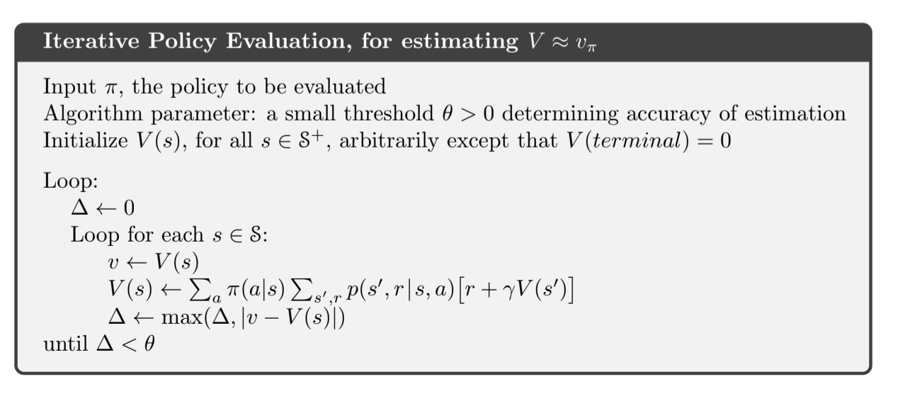Fig 4.1. Iterative policy evaliation

4.2. Policy Improvement

• We have a policy $\pi$ and we have determined the associated value function $v_{\pi}$ (with policy evaluation)
• For some state $s$ we would like to know it we should select action $a \neq \pi(s)$, a better action than the one currently advised by our policy
• One way to do this is to select $a$ and thereafter following the existing policy $\pi$:

$$\begin{equation} \label{eq5} \begin{split} q_{\pi}(s, a) & \doteq \mathbb{E}[R_{t+1} + \gamma v_{\pi} (S_{t+1}) | S_t = s, A_t = a]\\ & = \sum_{s',r} p(s', r | s, a) [r + \gamma v_{\pi}(s')] \end{split} \end{equation}$$

• If this quantity is greater than $v_{\pi}(s)$, it means it’s better to take action $a$ then follow $\pi$ than follow $\pi$ all the time
• This is a special case of the general result called policy improvement theorem

Policy improvement theorem

Let $\pi$ and $\pi’$ be two deterministic policies such that, $\forall s \in \mathcal{S}$:

$$q_{\pi}(s, \pi'(s)) \geq v_{\pi}(s)$$

Then the policy $\pi’$ is as good or better than $\pi$, meaning that the expected return is greater or equal for all states:

$$v_{\pi'}(s) \geq v_{\pi}(s)$$

Proof

1. Start from $q_{\pi}(s, \pi’(s)) \geq v_{\pi}(s)$
2. Expand the $q_{\pi}$ part with its expectation definition
3. Reapply the inequality until we have $v_{\pi’}(s)$

$$\begin{array}{rclr} v_{\pi}(s) & \leq & q_{\pi}(s,\pi'(s))\\ & = & \mathbb{E}_{p,\pi} [R_{t+1} + \gamma v_{\pi}(S_{t+1})\ |\ S_t{=}s, A_t{=}\pi'(s)] & \text{(by definition of } q_{\pi} \text{, with } \mathbb{E} \text{ starting in an action-node)}\\ & = & \mathbb{E}_{\pi',p,\pi} [R_{t+1} + \gamma v_{\pi}(S_{t+1})\ |\ S_t{=}s] & (\text{by starting } \mathbb{E} \text{ from the previous state node})\\ & \leq & \mathbb{E}_{\pi',p,\pi} [R_{t+1} + \gamma q_{\pi}(S_{t+1},\pi'(S_{t+1}))\ |\ S_t{=}s] & \text{(by applying the inequality } v_{\pi}(s) \leq q_{\pi}(s,\pi'(s)) \text{ to } S_{t+1} \text{)}\\ & \vdots & & \text{(by progressively combining all the } \mathbb{E} \text{ terms)}\\ & \leq & \mathbb{E}_{\pi',p} [R_{t+1} + \gamma R_{t+2} + \gamma^2 R_{t+3} + ... \ |\ S_t{=}s] & (\text{by reaching the end state, which removes } \pi \text{ from the equation)}\\ & = & v_{\pi'}(s) & \text{(by definition of } v_{\pi} \text{)}\\ \end{array}$$

Policy improvement

So far we saw how to evaluate a change in a policy in a single state on a particular action. The natural extension to this is to consider all states and all actions. In the greedy policy $\pi’$, we select at each state the action that appears best according to $q_{\pi}(s, a)$:

$$\begin{equation} \label{eq6} \begin{split} \pi'(s) & \doteq \underset{a}{\mathrm{argmax}}\;q_{\pi}(s, a)\\ & = \underset{a}{\mathrm{argmax}}\;\mathbb{E}[R_{t+1} + \gamma v_{\pi} (S_{t+1}) | S_t = s, A_t = a]\\ & = \underset{a}{\mathrm{argmax}}\;\sum_{s',r} p(s', r | s, a) [r + \gamma v_{\pi}(s')] \end{split} \end{equation}$$

• we take the action that looks best in the short term (one step lookahead) according to $v_{\pi}$
• if the new policy $\pi’$ is equally good but not better than $\pi$, then we have reached the optimal policy

4.3. Policy iteration

1. Take policy $\pi_n$ (meaning the policy at iteration $n$)
2. Compute $v_{\pi_n}$
3. Use $v_{\pi_n}$ to compute better policy $\pi_{n+1}$
4. Repeat until convergence

$$\pi_0 \overset{E}{\rightarrow} v_{\pi_0} \overset{I}{\rightarrow} \pi_1 \overset{E}{\rightarrow} v_{\pi_1} \overset{I}{\rightarrow} \pi_2 \overset{E}{\rightarrow} ... \overset{I}{\rightarrow} \pi_* \overset{E}{\rightarrow} v_{\pi_*}$$

Perks:

• Each policy is guaranteed to be a strict improvement of the previous one
• This process converges to an optimal policy and optimal value function in a finite number of steps (for finite MDPs)

Implementation

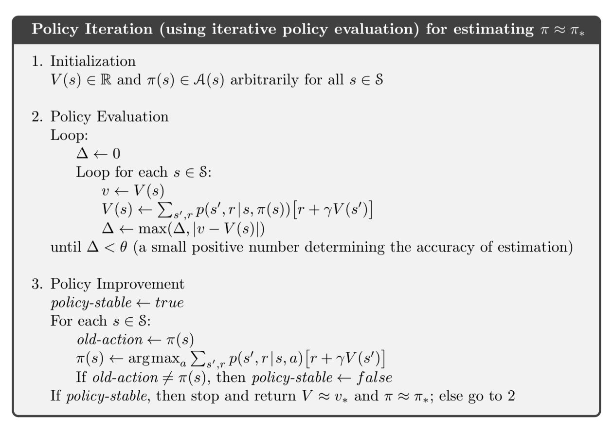Fig 4.2. Policy iteration

• Policy evaluation starts with the value function of the previous policy
• In production, we need to make sure the policy improvement doesn’t switch between two equally good policies

Policy iteration for action values

1. Initialization

$Q(s,a) \in \mathbb{R}$ and $\pi(s) \in A(s)$ for all $s \in \mathcal{S}, a \in \mathcal{A}$

2. Policy Evaluation

Loop:

$\Delta \gets 0$ Loop for each (s, a) pair:

$q \gets Q(s, a)$ $Q(s, a) \gets \sum_{s', r} p(s', r | s, a) [r + \gamma \sum_{a'}Q(s', a')]$ $\Delta \gets \mathbf{max}(\Delta, |q - Q(s,a)|)$

until $\Delta \lt \theta$ some threshold

3. Policy Iteration

is_stable $\gets$ true for each (s, a) pair:

$p \gets \pi(s, a)$ $\pi(s, a) \gets \mathbf{arg max}_{s,a}Q(s, a)$ if $p \neq \pi(s, a)$ then is_stable $\gets$ false

if is_stable then stop else goto 2.

4.4. Value Iteration

TL;DR: Ve’re trying to find optimal policy using policy iteration with one sweep of policy evaluation

Optimal policy (to build intuition about why value iteration works)

Any optimal policy can be subdivided into two components:

• An optimal first action $A_*$
• Followed by an optimal policy from successor state $S’$

Here we break down a definition of optimal policy in terms of finding an optimal policy from all the states that we can end up in.

Principle of optimality applied to policies: A policy $\pi(a|s)$ achieves the optimal value from state $s$, $v_{\pi}(s) = v_*(s)$, if and only if:

• for any state $s’$ reachable from $s$,
• $\pi$ achieves the optimal value from state $s’$

We’re going to use this to build value iteration:

• If we know the solution for subproblems $v_*(s’)$
• Then the solution $v_*(s)$ can be found by one-step lookahead $v_*(s) = \underset{a}{\mathcal{max}}\; \sum_{s’,r} p(s’, r|s,a) [r + \gamma v_*(s’)]$
• The idea of value iteration is to apply these updates iteratively
• Start with final rewards and work backwards

We know the optimal solution from the leaves and we back this up in the tree by maxing out of all the things we can do.

Value Iteration

• Every iteration of policy iteration involves policy evaluation to compute $V$
• Convergence to $V_{\pi}$ occurs only in the limit
• value iteration: policy evaluation is stopped after one sweep
• Simple update combining policy improvement and truncated policy evaluation:

$$\begin{equation} \label{eq7} \begin{split} v_{k+1}(s) & \doteq \underset{a}{\mathcal{max}}\; \mathbb{E} [ R_{t+1} + \gamma v_k(S_{t+1}) | S_t = s, A_t = a]\\ & = \underset{a}{\mathcal{max}}\; \sum_{s',r} p(s', r|s,a) [r + \gamma v_k(s')] \end{split} \end{equation}$$

• We are turning the Bellman optimality equation into an update rule
• Value iteration update is identical to policy evaluation update except here we max over all actions
• Each intermediate construct of $V$ doesn’t correspond to any policy

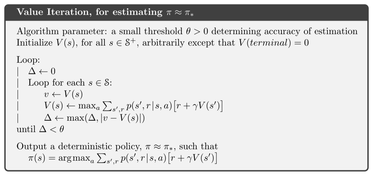Fig 4.3. Value Iteration

4.5. Asynchronous Dynamic Programming

• Major drawback of the methods we just saw: we always have to loop over the state space. If it’s huge, we’re screwed
• Asynchronous DP algorithms update value of states in any order, using whatever values for other states are available at the time of computation
• The order of the states that we will update will matter more (we might even try to skip useless states)
• Asynchronicity also makes it easier to intermix computation with interaction with the environment (which can guide the selection of states that we’ll update, for example we focus on the states we actually visit)
• Prioritize the selection of which state to update based to the magnitude in the Bellman equation error (more error: more priority)

4.6. Generalized Policy Iteration

• Process 1 - policy evaluation: make the current value function consistent with current policy
• Process 2 - policy improvement: make the policy greedy wrt the current value function
• In policy evaluation, these two processes alternate
• In value iteration, they don’t really alternate, policy improvement only waits for one iteration of the policy evaluation
• In asynchronous DP, the two processes are even more interleaved
• generalized policy iteration: let policy evaluation and policy improvement interact, independent of the granularity. When they stabilize, we have reached optimality.

Why? The value function stabilizes only when it is consistent with the current policy, and the policy stabilizes only when it is greedy with respect to the current value function. Thus, both processes stabilize only when a policy has been found that is greedy with respect to its own evaluation function. This implies that the Bellman optimality equation holds, and thus that the policy and the value function are optimal.

If improvements stop,

$$q_{\pi}(s, \pi'(s)) = \underset{a \in \mathcal{A}}{\mathbf{max}} \; q_{\pi}(s, a) = q_{\pi}(s, \pi(s)) = v_{\pi}(s)$$

Then the Bellman equation has been satisfied:

$$v_{\pi}(s) = \underset{a \in \mathcal{A}}{\mathbf{max}} \; q_{\pi}(s, a)$$

Both processes are:

• cooperating towards the same goal: optimality
• competing because making the policy greedy with respect to the value function typically makes the value function incorrect for the new policy

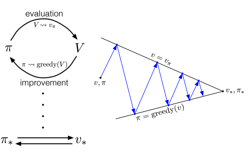Fig 4.4. GPI Interaction

4.7. Efficiency of Dynamic Programming

• If $n$ and $k$ are the number of states and actions, then there are $k^n$ policies
• DP methods have polynomial time, which is better than other methods
• Policy iteration and value iteration can be used up to a fair number of states, and asynchronous DP even more

4.8. Summary

Basic ideas for solving MDPs with Dynamic Programming:

• Policy evaluation refers to the (typically) iterative computation of the value function given a policy
• Policy improvement refers to the computation of an improved policy given the value function for current policy
• Putting these two together gives policy iteration and value iteration
• DP methods sweep through the state space, performing an expected update operation for each state
• Expected updates are Bellman equations turned into assignments to update the value of a state based on the values of all possible successor states, weighted by their probability of occurring
• GPI refers to the interleaving of policy evaluation and policy improvement to reach convergence
• Asynchronous DP frees us for the complete state-space sweep
• We update estimates of the values of states based on estimates of the values of successor states. Using other estimates to update the value of one estimate is called bootstrapping

Problem	Bellman equation	Algorithm
Prediction	Bellman Expectation Equation	Iterative policy evaluation
Control	Bellman Expectation Equation + Greedy Policy Improvement	Policy Iteration
Control	Bellman Optimality Equation	Value Iteration

• Algorithms are based on state-value function $v_{\pi}(s)$ or $v_*(s)$
• Complexity $O(mn^2)$ per iteration, for $m$ actions and $n$ states
• Could also apply to action value functions $q_{\pi}(s, a)$ or $q_*(s, a)$
• Would be $O(m^2n^2)$

DP requires a complete model of the environment, and does bootstrapping (i.e. creating estimates out of other estimates). In the next chapter (Monte Carlo methods) we don’t require any model and we don’t bootstrap. In the chapter after (TD-learning) we do not require a model either but we do bootstrap.