Sutton & Barto summary chap 06 - Temporal Difference Learning
This post is part of the Sutton & Barto summary series.
- 6.1. TD Prediction
- 6.2. Avantages of TD prediction Methods
- 6.3. Optimality of TD(0)
- 6.4. Sarsa: On-policy TD Control
- 6.5. Q-learning: Off-policy TD control
- 6.6. Expected Sarsa
- 6.7. Maximization Bias and Double Learning
- 6.8. Games, afterstates, and Other special cases
Temporal-Difference (TD) Learning is a combination of:
- Monte Carlo methods (can learn from experience without knowing the model)
- Dynamic programming (update estimate based on other learned estimates)
Each error is proportional to the change over time of the prediction, that is, to the temporal differences in predictions.
6.1. TD Prediction
MC waits until the return following the visit is known and then uses it as a target for $V(S_t)$. Every visit MC method:
where $G_t$ is th actual return following time $t$ and $\alpha$ a constant step-size parameter.
TD methods need only to wait until the next time step. At $t+1$ we use the observed reward $R_{t+1}$ and the estimate $V(S_{t+1})$ to create a target:
This method is called TD(0) or one step TD because it’s a special case of TD($\lambda$) which will be discussed in chapter 12 (eligibility traces) and chapter 7 (n-step bootstrapping).
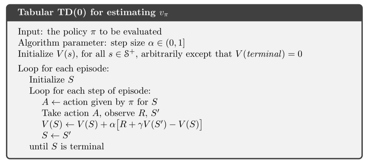
Fig 6.1.Tabular TD(0)
Because TD(0) bases its update on an existing estimate (as opposed to the real value), we say it’s a bootstrapping method, like Dynamic Programming (chapter 3). From this chapter we know:
Roughly speaking, MC uses an estimate of \ref{eq:6.3} as a target, DP uses an estimate of \ref{eq:6.4}. MC uses an estimate because the expected value is not known, and DP uses an estimate because $v_{\pi}(S_{t+1})$ is not known and we use $V(S_{t+1})$ instead. The TD target is an estimate for both reasons:
- it samples the expected values in \ref{eq:6.4}
- and it uses the current estimate $V$ instead of $v_{\pi}$
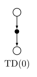
Fig 6.2.TD(0) backup
- The value estimate for the state node at the top of the backup diagram is updated on the basis of one sample transition from it to the immediately following state.
- Sample updates differ from expected updates of DP methods in that they are based on a single sample successor instead of a complete distribution over all possible successors.
- The quantity in brackets in \ref{eq:6.2} is a sort of error, measuring the difference between the estimated value of $V(S_t)$ and the better estimate $R_{t+1} + \gamma V(S_{t+1})$. This quantity is called the TD error and often written:
The TD error at each time is the error made at that time. $\delta_t$ is available at time step $t+1$
If the array $V$ does not change during the episode, then the MC method can be written as a sum of TD errors:
This identity is not exact if $V$ is updated during the episode (as in TD(0)), but if the step size is small it may hold approximately.
6.2. Avantages of TD prediction Methods
- they do not require a model of the environment
- online, fully incremental updates (no delay, no waiting for the end of the episode like Monte Carlo)
- for a fixed policy $\pi$, TD(0) has been shown to converge to $v_{\pi}$ (discussed in chapter 9)
- TD methods usually converge faster than MC methods
6.3. Optimality of TD(0)
Batch updating
Say we have a limited amount of experience. In this case a common approach is to present to experience repeatedly until the method converges. Given an approximate value function $V$, the increment in $V(S_t) \leftarrow V(S_t) + \alpha [R_{t+1} + \gamma V(S_{t+1}) - V(S_t)]$ is computed for every time step $t$ at which a nonterminal state is visited, but the value functon is only changed once, by the value of the increments. Then all the experience is presented again with the new value function to produce a new overall increment, and so on until convergence. We call this batch updating because updates are made only after processing each complete batch of training data.
Convergence
Under batch updating, TD(0) converges deterministically to a single answer given that $\alpha$ is sufficiently small. The constant-$\alpha$ MC also converges, but to a different answer. Understanding those differences will help understand the differences between the two methods.
Example 1 - Random walk under batch updating
After each new episode, all episodes seen so far are treated as a batch. They are repeatedly presented to the algorithm, either TD(0) or constant-$\alpha$ MC. The resulting value function was compared with $v_{\pi}$ and the average RMSE was plotted in figure 6.2:
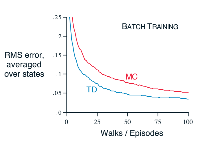
Fig 6.2. Performance of TD(0) and constant-$\alpha$ MC under batch training on the random walk task
- MC converge to values $V(s)$ that are sample averages of the actual returns experienced after visiting each state $s$.
- TD is optimal in a way that is more relevant to predicting returns
Example 2 - Markov reward process
- you want to predict the returns of an unknown markov reward process
- you observe the following episodes:
- A, 0, B, 0
- B, 1
- B, 1
- B, 1
- B, 1
- B, 1
- B, 1
- B, 0
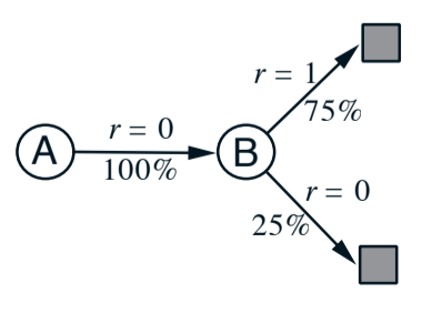
Fig 6.3. Markov reward process
- We can imagine the graph presented in fig 6.3
- For estimating V(B), we can agree that it’s $\frac{3}{4}$, based on the returns we’ve seen.
- But for V(A)?
- One answer is to consider that state A transitions 100% of the time into B so $V(A) = V(B) = \frac{3}{4}$. This is the answer batch TD(0) gives
- The other answer is to observe that we have seen A once and the return that followed was 0, so estimate V(A) = 0. This is what MC do.
The second method gives the minimum squared error on the training data (in fact 0 on training data) but we still expect the first answer to be better, since we expect it to be better on future data.
The difference between batch TD(0) and MC is that MC will always find the estimate that minimizes mean squared error on train data, whereas batch TD(0) always find the estimate that would be correct for the maximum likelihood model of the Markov process. In general, the maximum likelihood estimate of a parameter is the value of the parameter for which the probability of generating the data is greatest. Given the estimated model, we can compute the estimate of the value function that would be correct if the model would be exactly correct. This is called the certainty equivalence estimate because it is equivalent to assuming that the estimate of the underlying process was known with certainty rather than being approximated.
Certainty-equivalence estimate
These examples help explain why TD(0) converges faster than MC.
- in batch form, it computes the true certainty-equivalence estimate.
- non-batch TD(0) may be faster than MC because it is moving toward a better estimate (even if it’s not getting all the way there)
The certainty-equivalence estimate is in some sense an optimal solution, but it is almost never feasible to compute it directly. If $n = |\mathcal{S}|$ is the number of states, then forming the maximum likelihood estimates takes $O(n^2)$ memory and computing the corresponding value function takes $O(n^3)$ computational steps. It’s nice to see that TD can approximate this in $O(n)$, and in problems with a large state space, TD methods can be the only way to approximate the certainty equivalence solution.
6.4. Sarsa: On-policy TD Control
We still use the pattern of GPI, this time using TD methods for the evaluation or prediction part. As in MC, we have the exploration vs exploitation tradeoff and we’ll use on-policy and off-policy methods. Here we present an on-policy TD control method.
First, we learn an action value function, rather than a state value function. For an on-policy method we must estimate $q_{\pi}(s, a)$ for the current behavior policy $\pi$ for all $s$ and all $a$. We’ll use the same TD method as above for leaning $v_{\pi}$. Here is an episode:
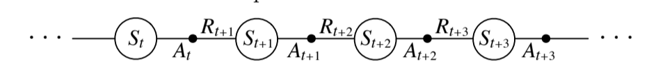
Fig 6.4. Sarsa
- previous section: we considered transitions from state-action pairs to states and learned the value of states
- now: we consider transitions from state-action pairs to state-action pairs, and learn the values of state-action pairs
Formally the two cases are identical, meaning that theorems assuring convergence of state value under TD(0) also holds for action values:
This update is done after every transition from a non-terminal state $S_t$. If $S_{t+1}$ is terminal, then $Q(S_{t+1}, A_{t+1}) = 0$ This rule makes use of five elements: $S_t, A_t, R_{t+1}, S_{t+1}, A_{t+1}$, hence the algorithm name.
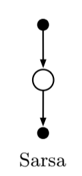
Fig 6.5. Sarsa backup
On-policy control algorithm
We continually estimate $q_{\pi}$ for the behavior policy $\pi$ and at the same time change $\pi$ towards greediness with respect to $q_{\pi}$
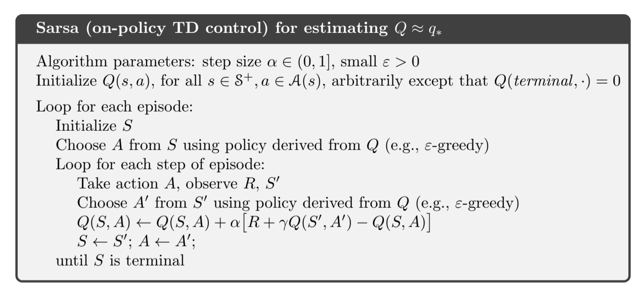
Fig 6.6. Sarsa algorithm
Convergence
Convergence properties of Sarsa depend on the nature of the policy dependence to Q. Sarsa converges with probability 1 to an optimal policy and action-value function as long as all the state-value pairs are visited an infinite amount of time and th policy converges in the limit to the greedy policy.
6.5. Q-learning: Off-policy TD control
Here the learned value function $Q$ directly approximates $q_*$, independent of the policy being followed.
The policy effect is to determine which state-action pairs are visited and updated. All is required for convergence is that all state-action pairs continue to be visited and updated.
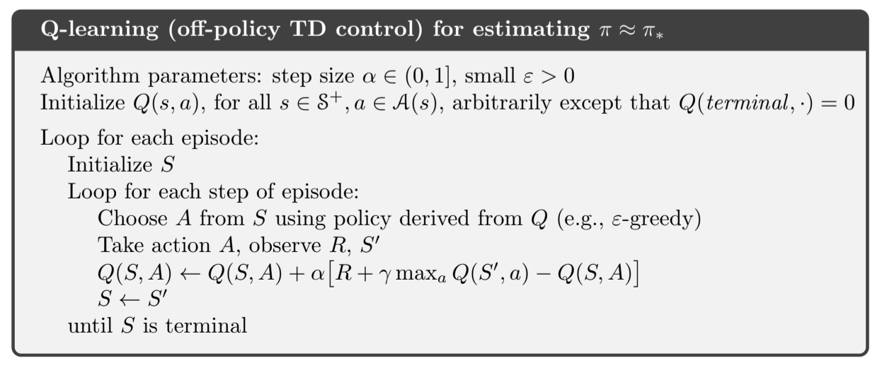
Fig 6.7. Q-learning
6.6. Expected Sarsa
Same as Q-learning except that instead of taking the max over the next actions we use the expected value, taking into account how likely each action is under the current policy.
Given the next state $S_{t+1}$, this algorithm moves deterministically in the same direction that Sarsa moves in expectation (hence the name).
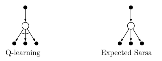
Fig 6.8. Backup diagrams for Q-learning and Expected Sarsa
It is more complex than Sarsa but removes the variance due to the random selection of $A_{t+1}$. Expected Sarsa might use a policy different from the target policy $\pi$ to generate behavior, becoming an off-policy algorithm. If $\pi$ is the greedy policy while behaviour is more exploratory, then Expected Sarsa is Q-learning.
6.7. Maximization Bias and Double Learning
All the control algorithms so far involve maximization in the construction of their target policy:
- in q-learning we use the greedy policy given the current action values
- in sarsa the policy is often $\varepsilon$-greedy
Maximization bias
In these algorithms, a max is implicitly used over the estimated values, which can lead to a significant positive bias. To see this, consider a single states $s$ in which for all actions the true value $q(s, a)$ is zero but whose estimated values $Q(s, a)$ are uncertain and thus distributed some above and some below zero. The max will always be positive, when the max over the true values is zero. It’s a maximization bias.
How to avoid maximization bias: double learning
One way to view the problem is that it is due to using the same samples (plays) both to determine the maximizing action and to estimate its value. Suppose we divide the plays into two sets and learn two independent estimates, $Q_1(a)$ and $Q_2(a)$, each an estimate of the true value $q(a)$.
- We use $Q_1$ to determine the maximizing action $A^* = \underset{a}{\mathrm{arg\,max}} \; Q_1(a)$
- We use $Q_2$ to provide an estimate of its value $Q_2(A^*) = Q_2 \; \underset{a}{\mathrm{arg\,max}} \; Q_1(a)$
This estimate will be unbiased in the sense that $\mathbb{E} [Q_2(A^*)] = q(A^*)$. We can reverse both to produce another unbiased estimate $Q_1(A^*) = Q_1 \; \underset{a}{\mathrm{arg\,max}} \; Q_2(a)$, and we have double learning.
Double q-learning
The idea of double learning extends naturally to algorithms for full MDPs. For example, Double Q-learning, divides the time steps in two, and with probability 0.5 the update is:
and with probability 0.5 the update is reversed, updating $Q_2$ instead.
- The behavior policy can use both estimates (an $\varepsilon$-greedy policy could be base on the average or sum of $Q_1$ and $Q_2$)
- There are also double versions of Sarsa and Expected Sarsa
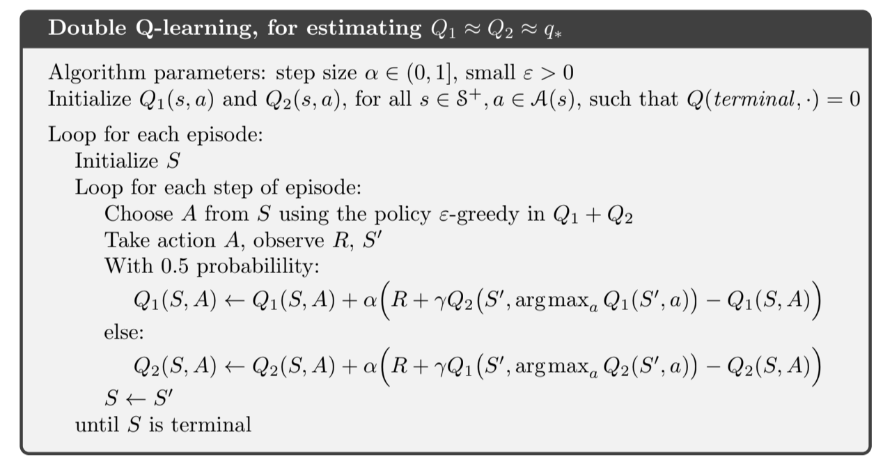
Fig 6.9. Double Q-learning
6.8. Games, afterstates, and Other special cases
In chapter 1 we presented a TD algorithm for learning Tic-Tac-Toe. It learned something more like a state-value function, but it’s neither an action-value nor a state-value in the usual sense. In a conventional state, the player has the option to play actions, but in tic-tac-toe we evaluate after the player has taken the action. It’s not an action-value either because we know the state of the game after the action is played. Let’s call these afterstates and the value functions over these afterstate value-functions
We can use these to valuate values more efficiently (in tic-tac-toe, two separate state-actions produce the same after state so we can just learn once on the afterstate and not on the two action-states)