Sutton & Barto summary chap 03 - Finite Markov Decision Processes
This post is part of the Sutton & Barto summary series.
- 3.1. Agent-environment interface
- 3.2. Goals and rewards
- 3.3. Returns and Episodes
- 3.4. Unified notation for Episodic and continuing tasks
- 3.5. Policies and value functions + Bellman equations
- 3.6. Optimal values and optimal policies
- 3.7. Optimality and approximation
- 3.8. Summary
3.1. Agent-environment interface
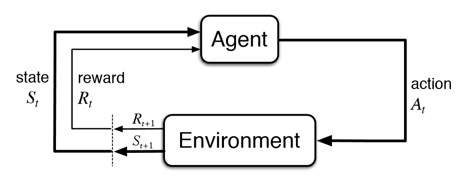 Fig 3.1. Agent and Environment interactions
In a finite MDP, the sets of states, actions and rewards are all finite.
The random variables $S_t$ and $R_t$ have well defined discrete probability distributions dependent only on the preceding state and action.
For particular values $s’$ and $r$, there is a probability of these values occurring at time $t$, given particular values of $s$ and $a$:
The function $p$ defines the dynamics of the MDP.
The MDP framework is very versatile, practically anything can be considered an action, a state or a reward. In general, anything that cannot be changed arbitrarily by the agent is considered part of the environment, but the environment is not necessarily totally unknown to the agent.
The “Markov” part in “Markov Devision Process” comes from the Markov property, which states that the future states of the process ($S_{t+1}$) only depends on the present state of the process ($S_t$). It means that the history leading to $S_t$ has no influence on $S_{t+1}$, all the information needed is embedded in $S_t$.
3.2. Goals and rewards
- At each time step the reward is a simple number $R_t \in \mathbb{R}$
- The goal of the agent is to maximize cumulative reward in the long run
- We can use the reward signal to give prior knowledge about how to achive the task
3.3. Returns and Episodes
Episodic case
- Simple definition of the expected return we want to maximize : $G_t = R_t + R_{t+1} + … + R_{T}$
- We get a reward at each time step, $T$ is the final time step
- This approach only makes sense when there is the notion of a final time step, that is when the agent actions naturally break into sequences, that we call episodes.
- Each episode ends in a special state called the terminal state.
- It’s important that the start of the episode is independent from the end of the previous episode.
- Tasks with episodes of this kind are called episodic tasks. In these, $S$ is the set of all nonterminal states, and $S^+$ is the set of all states including terminal ones.
Continuous case
- When the agent-environment interaction does not naturally break into episodes
- The final timestep is $\infty$ so we can’t really compute a useful $G_t$
- We introduce discounting: $G_t = R_{t+1} + \gamma R_{t+2} + \gamma^2 R_{t+3} + … = \sum_{k=0}^{\infty} \gamma^k R_{t+k+1}$
- $0 \leq \gamma \leq 1$, (for $\gamma = 0$ the agent is myopic)
3.4. Unified notation for Episodic and continuing tasks
- We use $S_t$ in the episodic case because the number of the episode considered is often explicit
- The return over a finite number of terms of the episodic case can be treated as the infinite sum by adding an absorbing state:
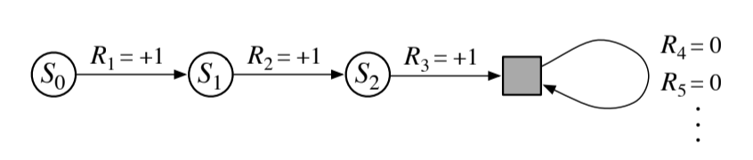 Fig 3.2. Addition of an absorbing state
Unified notation for the return, that includes the possibility of $T = \infty$ or $\gamma = 1$:
3.5. Policies and value functions + Bellman equations
- value function: expected return in a state (or a q-state for q-values // q-state is (s, a))
- policy: mapping from states to probabilities of taking each possible action
- Reinforcement learning methods specify how the agent’s policy is changed as a result of its experience
The value function of a state $s$ under a policy $\pi$, denoted $v_{\pi}(s)$, is the expected return starting in $s$ and following $\pi$ thereafter.
Same for the action-value function $q_{\pi}$:
$v_{\pi}(s)$ and $q_{\pi}(s)$ can be determined by experience. If we maintain an average reward received for each state (or q-state), this average converges to $v_{\pi}(s)$ (resp $q_{\pi}(s)$). If there are too many states, we would have to maintain $v$ and $q$ as parametrized functions instead, and adjust the parameters to better match the observed returns.
Value functions also have a nice recursive property:
It can be viewed on a sum on 3 values $a, s’$ and $r$. For each triple we compute the probability $\pi(a|s) \; p(s’, r | s, a)$, weight the quantity in brackets by this probability, then sum over all the probabilities to get an expected value.
This is the Bellman equation for $v_{\pi}$. It expresses a relationship between the value of a state and the values of its successor states.
We can represent this with a backup diagram. It’s called backup diagram because they visualize the operations that transfer values back to a state from its successor states.
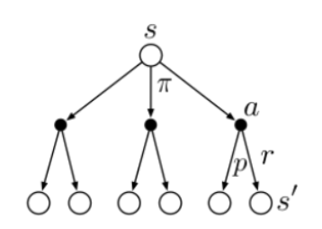 Fig 3.3. A backup diagram
When we are at the root node $s$, the Bellman equation averages over all the possibilities under this node, weighting each by its probability of occurring. The value of the start state must be equal to the discounted value of the expected next state, plus the reward we got along the way.
The value function $v_{\pi}$ is the unique solution to its Bellman equation and this forms the basis of a number of ways to compute, approximate, and learn $v_{\pi}$.
Bellman equation for $v_{\pi}(s)$
A state-value is an expectation over the available action-values under a policy:
[*] Given a state-action pair, the return $G_t$ is an action-value. In the example above: $G_t$ is a function of the state $s$ (given by the condition “$S_t{=}s$”) and the action $A_t$ (given by the policy $\pi$ under the expectation “$\mathbb{E}_{\pi,p}$”).
The following recursive relationship satisfied by $v_{\pi}(s)$ is called the Bellman equation for state-values. The value function $v_{\pi}(s)$ is the unique solution to its Bellman equation.
In summary:
Fig 3.4. Backup diagram for $v_{\pi}$
Bellman equation for $q_{\pi}(s,a)$
An action-value is an expectation over the possible next state-values under the environment’s dynamics.
[*] Given only a state $s$, the return $G_t$ is a state-value. In the example above: $G_t$ is a function of the state $S_{t+1}$ (given by the environment’s dynamics $p$ under the expectation “$\mathbb{E}_{p,\pi}$”).
The following recursive relationship satisfied by $q_{\pi}(s,a)$ is called the Bellman equation for action-values. The value function $q_{\pi}(s,a)$ is the unique solution to its Bellman equation.
In summary:
 Fig 3.5. Backup diagram for $q_{\pi}$
3.6. Optimal values and optimal policies
The Bellman equation shows us how to compute the value of a state for a any policy $\pi$. The Bellman optimality equations focus on the optimal policy.
- $\pi \geq \pi’$ iif $v_{\pi}(s) \geq v_{\pi’}(s)\;\; \forall s \in S$
- the optimal policy is $\geq$ to all other policies
- the optimal functions are called $v_*$ and $q_*$
For a state-action pair, the optimal function gives the expected return for taking action $a$ in state $s$ and thereafter following an optimal policy.
Bellman optimality equations
It expresses the fact that the value of a state under the optimal policy must equal the expected return for the best action from that state:
The last 2 equations are the forms of the Bellman optimality equations for $v_*$.
For $q_*$ we have:
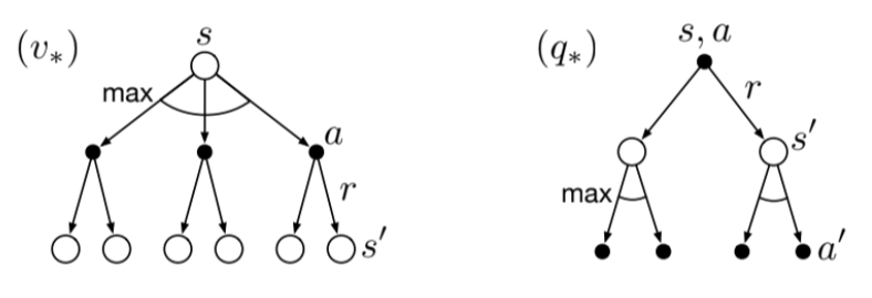 Fig 3.6. Backup diagrams for $v_*$ and $q_*$
- For finite MDPs, the Bellman optimality equation for $v_*$ has a unique solution
- It’s a system of equations, one for each state (one unknown for each state)
- If the dynamics of the system are known we can solve this using any nonlinear system solving method
- Once we have $v_*$, it’s easy to find the optimal policy (greedy with respect to the optimal evaluation function $v_*$)
- It’s even easier if we have $q_*$ because we just take the max without even having to do the one-step lookahead (i.e using the environment’s dynamics - the $p$ function - , which we often do not have)
But this solution relies on 3 principles that are rarely true in practice:
- we acurately know the dynamics of the environment
- we have enough computational resources to compute the solution
- the Markov property
3.7. Optimality and approximation
- We have defined what are optimal value functions and optimal policies
- For most practical cases, it is very difficult to compute a truly optimal policy by solving the Bellman equation, even if we have an accurate model of the environment’s dynamics
- In a practical setting we almost always have to settle for an approximation. But we can do this in a clever way: making approximate optimal policies that play nearly optimally in regions of the state space that are actually encountered, at the expense of making very poor decisions in the states that have a very low probability of occuring.
3.8. Summary
- Reinforcement Learning is about learning from interaction how to behave to achieve a goal
- Everything inside the agent is completely known and controllable
- Everything outside the agent is incompletely controllable and may or may not be completely known
What we saw:
- What a policy is
- The notion of return return (possibly with discount, denoted $\gamma$)
- A policy’s value function $v_{\pi}$ assign to each state the expected return for that state
- The Bellman equations express $v_{\pi}$ and $q_{\pi}$
- The Bellman optimality equations express $v_*$ and $q_*$, following the optimal policy
- Need for approximated solutions