Structured bandits for healthcare
This post is part of a series of blogposts about the lectures we had at the Reinforcement Learning Summer School (RLSS) 2019.
- RL needed reminders
- Optimizing super-resolution imaging parameters
- Adaptive clinical trials
- Conclusion
On the second day of RLSS we started having ‘short’ (~1h) talks about various application of RL from people actually working in the industry. For that first session Audrey Durand was here to present her work with RL in healthcare. As usual for my posts about RLSS, the material is not my own (slides can be found here) and I’m just compiling my summary here. I found this talk great not only because of the applications shown, but also by the clarity of the explanations about which parts of RL are used since it’s a really nice (partial) summary of the previous lectures.
RL needed reminders
In this talk we are going to see an application of bandits in the context of healthcare. Two kind of stochastic bandits will be presented:
- structured bandits applied to imaging parameter tuning for neuroscience
- contextual bandits for adaptive cancer treatment in mice
As a reminder, the talk begin with useful definitions of RL that will be used in this setting. We are in the setting of stochastic multiarmed bandits, and at each timestep $t$ we select an action $k_t \in {1, 2, … K}$ which correspond to selecting arm $k$. We then observe the outcome $r_t$ that is drawn from a distribution with mean $\mu$ of the arm we pulled at time $t$: $r_t \sim D(\mu_{k_t})$.
In RL, we try to maximize an expected reward. To do that in the context of bandits, we need exploration to make sure we don’t converge to a bad arm and we also need to exploit our current knowledge of which are is good or bad in order to not try too often arms (actions) that we think are bad (i.e. minimize the regret $R(T) = \sum_{t=1}^T [\mu_{k^*} - \mu_{k_t}]$).
As we have learned in the previous lectures of the RLSS (blogposts coming soon), we have many strategies to do exactly that while having sublinear regret. This last notion is important because if an algorithm gives linear regret (linear with respect to iterations $t \in T$), we are not really learning anything. We want algorithms that give sub-linear regret to capitalize on our experience.
Some of these strategies include:
- $\epsilon$-greedy
- Optimism in front of uncertainty (UCB)
- Thompson sampling
- Best Empirical Sampled Average (BESA)
All these strategies come with their guarantees, essentially they show sublinear regret (either $\sqrt(t)$ or $\log(t)$) under the proper assumptions. In practice sometimes these assumptions may not be true but that doesn’t mean we cannot have good performance, it just open new problems.
In practice we can’t compute the regret since it requires knowing the true mean $\mu_{k^*}$, which we obviously don’t have because if we did we wouldn’t be doing all of this in the first place. Instead, we can:
- minimize bad events so that we accumulate them sublinearly. (In real life that could be bad patient outcomes!)
- maximize cumulative good events
This doesn’t make practice not interesting nor theory irrelevant, because all these disparities between practice and theory will be good opportunities to face new constraints and challenges that are relevant to the application, and gives incentive to bandit researchers to addressing new problems.
Structured bandits
One of the settings that arise when we want to apply bandits in practice is the case where we have a big number of actions. now we can’t treat the problem like a normal bandit otherwise it would take too much time before converging because we need to try all the actions enough times to converge.
One solution to this problem is to assume there is some kind of structure underlying our action space. We are going to exploit this structure in order to learn faster, by sharing information across the actions.
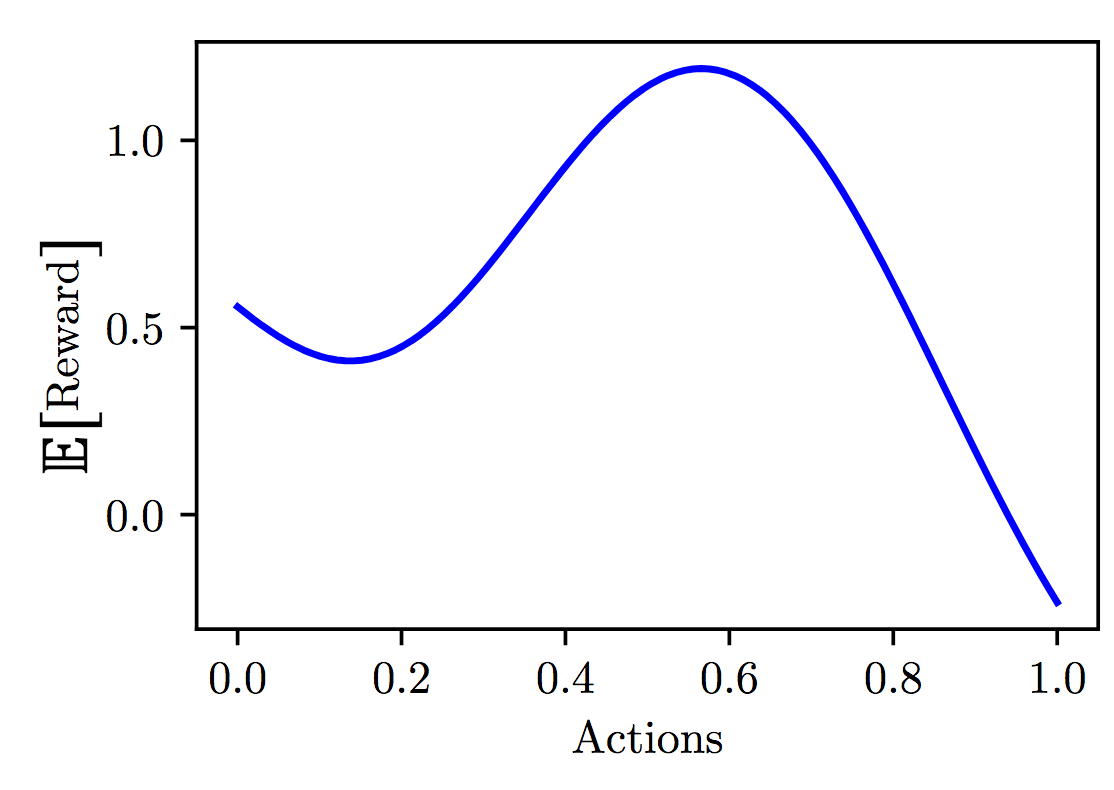 Fig 5.1. Structure in actions. Source: Audrey Durand
As a quick recap of the structure bandits lecture (coming soonTM), in the structured bandit setting, instead of having an independent mean $\mu_k$ per action (represented as the x-axis on figure 5.1), our actions are now represented by features $\mathcal{X}$ and our expected reward is a function of these features $f: \mathcal{X} \mapsto \mathbb{R}$. Now the ‘player’ of the bandit has access to this action space $\mathcal{X}$ and at each episode $t$ we take an action $\mathcal{X}_t$ and we observe a reward sampled from a distribution which expected payoff is given by $f(\mathcal{X}_t)$.
Capturing structure
Linear model
Our goal still to maximize the reward which can now be formulated as finding $\mathcal{X}^* = \mathrm{argmax}_{x \in \mathcal{X}} f(x)$. One way to do this as seen in the previous lecture is to capture the structure using a linear model. Not necessarily a model linear on the inputs directly but it can be linear on a feature mapping ($\phi$) of the inputs.
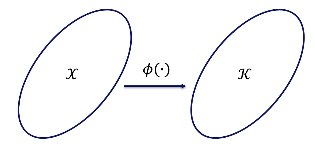 Fig 5.2. Linear model. Illustration of the mapping $\phi$. Source: Audrey Durand
In this setting we’ll assume our function $f$ is associated with some unknown parameters $\theta$ and the value of $f$ at any point $x$ can be recovered as being the inner product between this parameter vector $\theta$ and the mapping $\phi$ from the action features $x$ to the space $\mathbb{R}^d$ that has the same dimension as the parameter vector $\theta$.
Then we can solve it with least squares in order to recover the function. We end up in an online function approximation problem where our goal is to estimate $\theta$ because if we have it then at any given point $x$ we would be able to recover $f(x)$ using the mapping $\phi$, so we would be able to pick the location $x^*$ in the action space that maximizes $f$.
In this setting we assume the observations are Gaussian so each time we select an action $x_t$ we observe an outcome that is $y_t = f(x_t) + \xi_t$ that include Gaussian noise $\xi_t \sim \mathcal{N}(0, \sigma^2)$.
The regret we want to minimize is the same as before except now we have $f(x)$ instead of $\mu$:
Kernel regression
In the case where the mapping $\phi : \mathcal{X} \mapsto \mathbb{R}^d$ can be expressed directly (= the dimension $d$ is not too large) we can solve the previous problem and find $x^*$ using least squares. In the case where we don’t have the mapping or its dimension $d$ is too large (even infinite), we can use kernel regression instead.
We assume we have some kernel function (\ref{eq:5.4}) that can give us some kind of similarity measure between two points $x$ and $x’$. This similarity is essentially the following inner product:
- We put a Gaussian prior on $\theta$: $\theta \sim \mathcal{N}(0, \Sigma)$ with $\Sigma = \frac{\sigma^2}{\lambda} I$, $\lambda > 0$ being the noise here.
- We can obtain the posterior distribution of the function $f$ in closed form using the ground matrix of the previous observations ($N$ is the number of previous observations):
\ref{eq:5.5} corresponds to the kernel applied to all the pairs of previous observation (that’s the ground matrix), and \ref{eq:5.6} is the vector of kernels between a new point $x$ that we want to evaluate and any previous observation $x_i$.
The posterior distribution on the expected function $f$ is given by a normal distribution parametrized by the posterior mean and the posterior variance:
This is essentially the kernel version of what we saw in the linear model where we don’t have to express the mappings $\phi$ anymore. It’s useful because in some cases it’s easier to have access to a kernel compared to having the mapping.
If we have a posterior like in \ref{eq:5.7}, we can sample functions from it (instead of sampling real numbers) because the posterior is fully defined (we have the posterior mean and covariance). As any typical posterior distribution, the more observations we have, the tighter the posterior variance is going to be around the posterior mean and this posterior mean is going to become closer to the true mean.
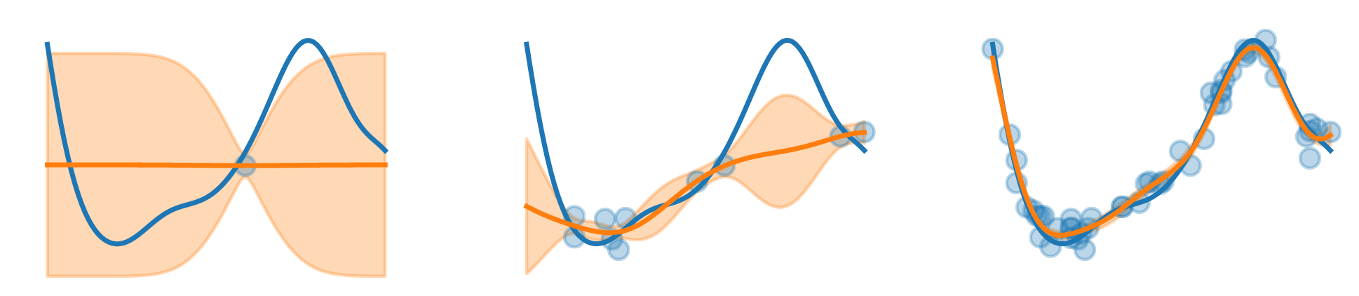 Fig 5.3. Illustration of the evolution of posterior functions using the defined posterior mean and standard deviation. Source: Audrey Durand
Streaming kernel regression
We are in the streaming kernel regression setting because our input locations are not independent. We can’t reuse any kind of algorithm because inputs are correlated with each other. Some algorithm work under that assumption such as Kernel UCB, Kernel Thompson Sampling, Gaussian Process UCB, Gaussian Process Tompson sampling.
Optimizing super-resolution imaging parameters
 Fig 5.4. Cervo research center logo.
After this very useful summary of structured bandits, we see how it is applied in a real world setting. As Audrey was mentioning in the talk, this application was done with the Servo research center (fig 5.4) in collaboration with a team of neuroscientists that look into the brain to understand it in order to understand more the processes involved in some diseases like Alzheimer or Parkinson’s.
Problem
In order to study the brain, these neuroscientists have to look at images of the brain, like figure 5.5 which represents a very neat picture of neurons where we see the ring structure corresponding to the actin protein that plays a role in the plasticity of the neurons.
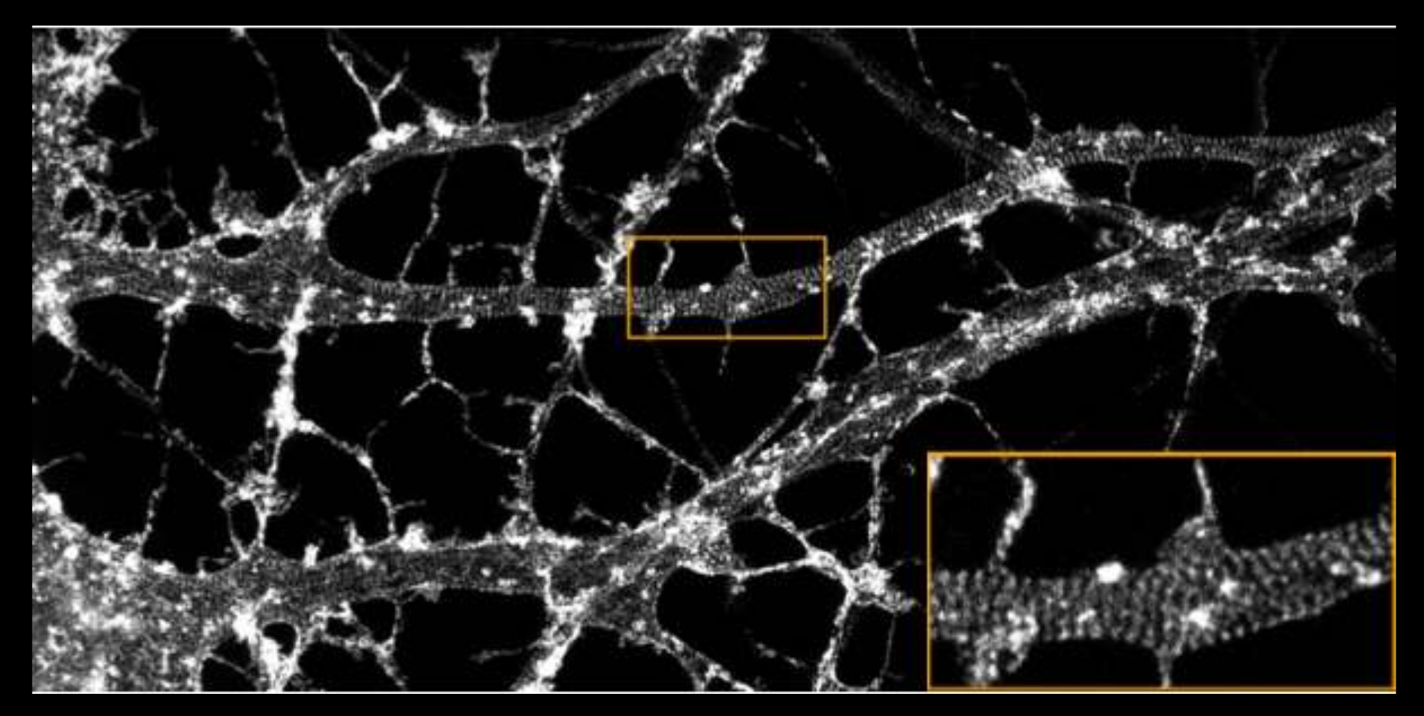 Fig 5.5. Picture of neurons with Actin rings structure highlighted. Source: Audrey Durand
Neuroscientists want to see how this protein behaves under different conditions to shed some light on how the brain evolves when it ages or under some conditions. Those images like in figure 5.5 are taken with very expensive devices (there are only a few of them in the world), and they are very hard to use to get good images. They are very hard to tune and without extensive knowledge of the machine and the sample one will usually picture useless noise.
It would be great to tune it once and then take many pictures but unfortunately the tuning also depends on the samples. The neurons are going to react differently to the picturing process in the image.
In practice, scientists divide their samples of the same batch into two groups, one that will be ‘sacrificed’ for tuning the machine and the other to take the actual pictures. The samples in the ‘tuning’ group cannot be reused to make proper images after because the imaging process uses lasers that can destruct the sample (photobleaching) during the tuning phase. This obviously has a lot of problems because we loose a lot of samples (which are from mice) and a lot of time.
Structured bandit modelisation
The solution would be to tune these parameters online in a structured bandits way, to reduce the amount of wasted samples. It’s a good usecase for structured bandits:
- We want to maximize the acquisition of good images (by finding the best parameters)
- minimize trials of poor parameters to avoid wasting samples.
We need some kind of feedback, and here it is going to be a representation of image quality, which is initially evaluated by a researcher putting a quality score on the images, well aware that this value should be as informative as possible. Figure 5.6 shows examples of bad images and good images, and all of these may have different scores, not just 0 for bad images and 1 for good ones.
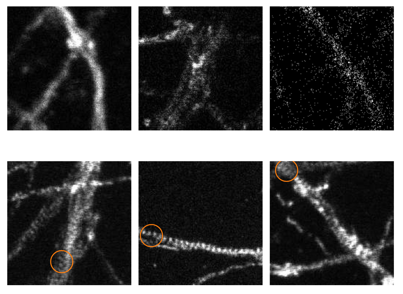 Fig 5.6. Examples of 'Bad' images (top row) and 'good' images (bottom row). Note the visible structure of Actin on good images. Source: Audrey Durand
Thompson sampling to generate imaging parameters
The strategy used to generate the imaging parameters was Thompson sampling. If we have a full posterior distribution on our function (like what can be obtain by kernel regression or gaussian processes), we can do Thompson sampling from that by sampling a function from the posterior and play according to that function (i.e. try to maximize the function).
Figure 5.7 shows an example of what can be obtain using Thompson sampling:
 Fig 5.7. Illustration of Thompson sampling for selecting imaging parameters. Source: Audrey Durand
The blue line is the true function, the orange line is the posterior and when we get more samples we can fit better the true function, and we will play (= select actions) according to the computed function.
Thompson sampling to generate outcome options
The Thompson sampling method managed to maximize the function and get good imaging parameters, but the major issue is that imaging can be a destructive process. In many cases, we want to take several pictures of the same sample before and after some treatment to see the evolution of the sample. This is not possible if the parameters of the machine are destructing every sample by photobleaching even if we get good quality images. We have to tradeoff image quality and photobleaching (multi-objective function).
The neuroscientists didn’t have an explicit function to combine these objectives into one so they put back the expert in the loop to evaluate the parameters proposed by the system to make that tradeoff. The goal of the algorithm is now not to produce parameters for the machine directly but to generate a set of different parameters with possible outcomes in terms of image quality and photobleaching levels. The expert would then look at the tradeoff only (not the parameters) and make a choice. To be able to explore, we have to add some noise in order to ‘trick’ the expert into choosing some optimistic tradeoff. Figure 5.8 shows the cloud of tradeoff options.
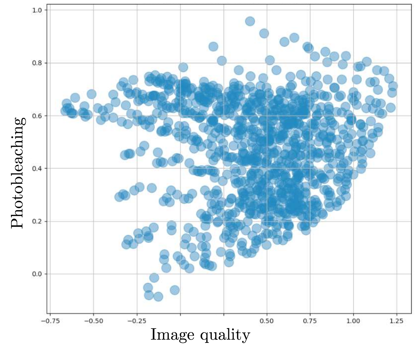 Fig 5.8. Photobleaching / image quality tradeoff possible outcomes. Source: Audrey Durand
Experiments and results
The first experiment shown in the presentation was tuning 3 parameters (1000 possible configurations), on 3 different image types:
- Neuron: rat neuron;
- PC12: rat tumor cell line;
- HEK293: human embryonic kidney cells
The experimental setup was to first take a non super-resolution image that is non-destructive but without enough quality to see meaningful structure, and then they would acquire two super-resolution images with the goal of improving image quality significantly without damaging the sample. Results are shown in figure 5.9.
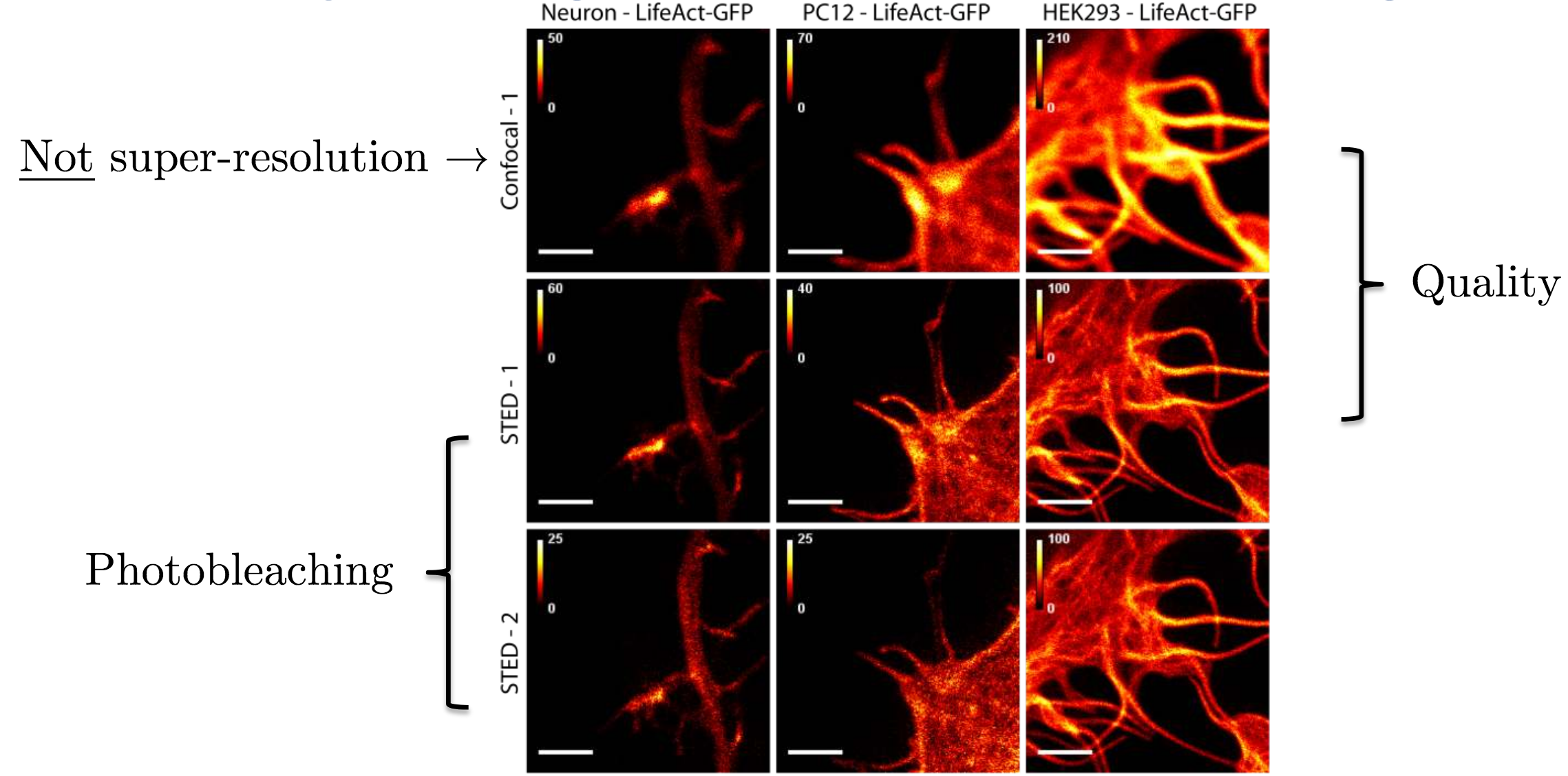 Fig 5.9. Experiment results for 3 different image types. We can see that the structure is much more visible on the super-resolution images. Source: Audrey Durand
Regret-wise, the results are also good. We don’t have access to the true regret but we can accumulate the occurrences of bad events (photobleaching or low quality images). Results are shown on figure 5.10 and we have sub-linear curves that validate the theory.
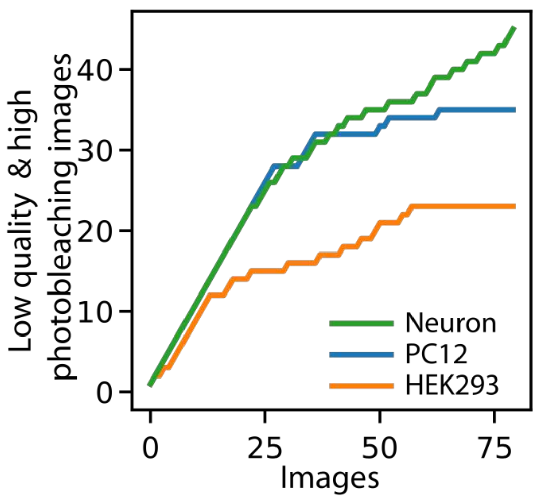 Fig 5.10. Regret-like curve showing sublinear convergence. Source: Audrey Durand
Fully automated process
The good results motivated the next phase of this work which was to automate the steps where a human expert was needed. Having collected many samples from the human expert, the team used this gathered data to train neural networks to do the quality analysis and the optimization parameter choice. On figure 5.11 we can see results of imaging before those networks parameters optimization, and after optimization, showing the success of this replacement.
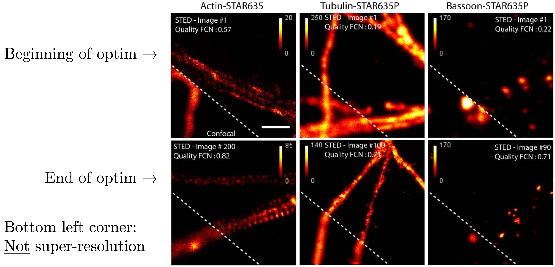 Fig 5.11. Images before and after neural network optimization. Source: Audrey Durand
Adaptive clinical trials
This second application of RL in healthcare goes closer to the patient by looking at randomized trials application for treatment comparison.
Randomized vs adaptive trials
Both of these trials are a way to compare treatments in healtcare. Let’s say we have a bunch of patiens, two treatments, and for the randomized trial we are going to separate the group into two parts randomly and assign treatment 1 to group 1, and treatment 2 to group 2. By the end of the study we can compare the results in both groups and make some conclusions about the treatment.
This is an ok method if we have many people and few treatments, but this is not always the case. Even in the perfect conditions, randomized trials means that the same amount of people getting the best treatment also get the worst treatment because our group is split into. Same thing with $k$ groups, $\frac{1}{k}$ people will get the best treatment and the same proportion will get the worst one. We would like a more adaptive solution where more people get the best option and only few people get the worst option, with a range of proportions in between.
A way to do that is through adaptive trial where we don’t fix all the study parameters before the study but instead adapt the design so that the probability of getting assigned the treatment depends on previous results of the treatment.
Contextual bandits
In this setting, treatments are our arms and their means $\mu$ are the probabilities that the treatments are effective. Patients are episodes, for each episode we select a treatment $k_t \in {1, 2, … K}$ and observe an outcome $r_t \sim D(\mu_{k_t})$.
When the patiens can be separated into groups (say men and women) to see if the treatment differs between groups, we can see these characteristics as contexts for contextual bandits. We can effectively treat them as two separat bandit problems that only depend on context. If th number of contexts grow very large, we face the same problem as in the previous bandit setting where the action space was very large.
Solution: exploit the structure on the context space.
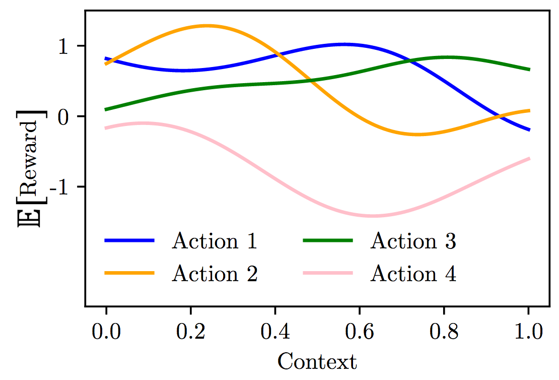 Fig 5.12. Contextual bandit setting where we try to leverage the structure of each context. Source: Audrey Durand
Each action will not have its own mean $\mu_k$, it will have a specific mean depending on the function of the context. The formulation of the bandit problem can be summarized as follows:
- The expected reward of action $k$ is a function $f_k$ of the context: $f_k: \mathcal{S} \mapsto \mathbb{R}$
For each episode $t$ (= each patient):
- Observe a context $s_t \sim \Pi$
- Select an action $k_t \in {1, 2… K}$
- Observe a reward $r_t \sim D(f_{k_t}(s_t))$
Our goal is to maximize the reward so to find:
Online function approximation
The problem described above is some sort of online function approximation problem, we are going to treat it under the linear model and solve it using kernel regression or gaussian processes as seen before in the structured bandits.
Before we had the function and actively pick the action that maximizes that function $f$. Here it is different, we have $k$ functions and we want to pick the action that has the highest value given a fixed given context.
Experiment formulation
Experiments on this setting were conducted on mice in collaboration with cancer researchers in Cyprus, and dedicated to compare several treatments:
- None: not treating (sometimes the body needs to rest)
- 5FU: this is chemoterapy
- Imiquimod: immunotherapy
- 5FU + Imiquimod
The mice were induced cancer tumors and the treatment given twice a week. The question is: which treatment should be allocated to the patient given the state of the disease, which in this case is approximated by the size of the tumor.
- Phase 1 of the experiment: exploration only by randomly assigning treatments and gathering data. Very few data could be collected for larger tumors because they would grow exponentially, leading to early death of the mice before collecting enough data.
- Phase 2: adaptive trial: adapt treatment allocation based on previous observations to have slower tumor growth and allow more data gathering for treatments
This second phase was designed as a contextual bandit problem:
- Improve treatment allocation online
- Maximize the amount of acquired data
- Minimize the allocation of poor treatments
We have to relax one of the assumption given in contextual bandits theory, because in practice in this experiment the contexts (tumour volume) are not independent on the actions (treatments given)!
To define the reward, we could go with the “natural” approach and say that the reward is the tumour volume reduction:
But it would not take into account the fact that smaller tumours are better than big ones so a better reward is:
Exploration / Exploitation strategy
The strategy used in the experiment was BESA (Best Empirical Sampled Average) extended to Gaussian Processes. The researchers would subsample the observations to make sure the regression model for each of the actions would be applied to the same number of observations. Figure 5.13 shows the different posterior means obtained by conditioning the posterior mean on different subsets of observations.
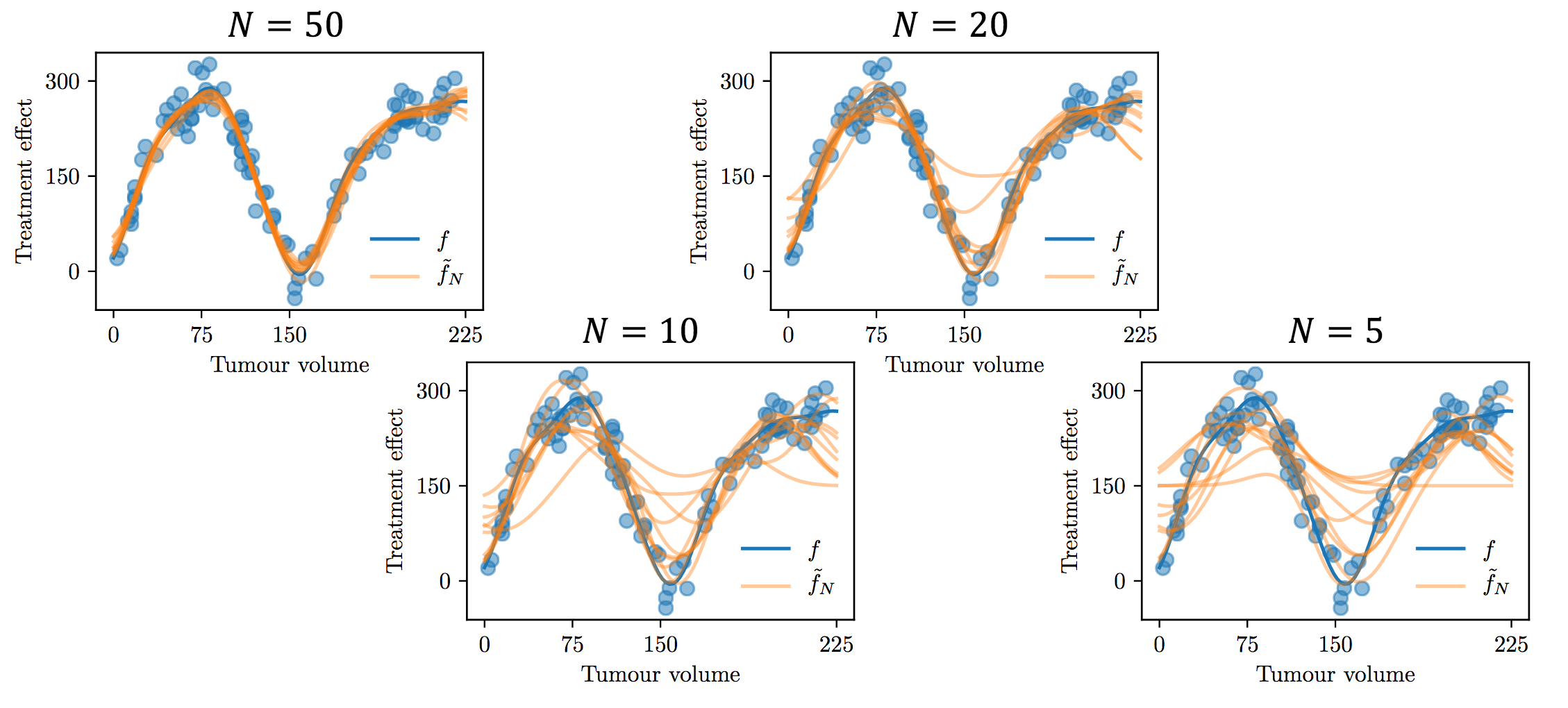 Fig 5.13. Subsampling of the observations to observe effect on the posterior mean. Each orange curve is a different posterior mean fitted on a subsample of size N of 100 observation points. Source: Audrey Durand
Unsurprisingly, the smaller the subsample, the more variance we get on the posterior means fitted on those points. This is where our exploration / exploitation is going to come from. Figure 5.14 shows an example for this exploration / exploitation strategy:
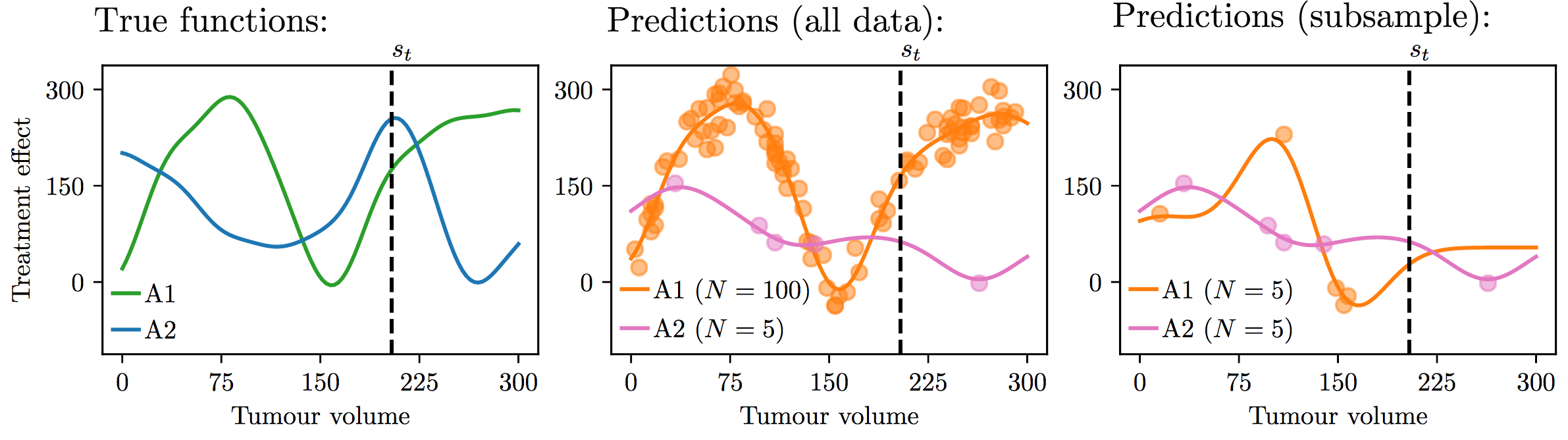 Fig 5.14. Exploration / exploitation strategy example. Source: Audrey Durand
In this example, the first graph shows two true functions. Here at a given context $s_t$ the optimal action would be action 2. On graph 2 we look at the kind of posterior means that we get by conditioning on $100$ points for action 1 and $5$ points for action 2 because it didn’t seem to work well in the beginning. With this estimation we are going to predict action 1 by keeping exploiting. If we subsample from these 100 observations for action 1 and take as much observations as action 2 ($N = 5$) we could get for example graph 3 in which the posterior mean forces us to explore at that point, making us pick action 2.
Phase 2 experiments and results
The researchers applied this setting on a sample of mice and undergo the adaptive treatment twice a week. Mice are separated into 4 groups, get treatment, and gather data at the ‘end’ (=death) of the group. The algorithm is updated at the end of a group for next group. So we get 4 updates in 4 episodes.
The results are promising, as in figure 5.15 we can see that the mice actually live longer at the end of the experiment, with lower variance which could mean convergence towards a strategy that is mostly exploiting.
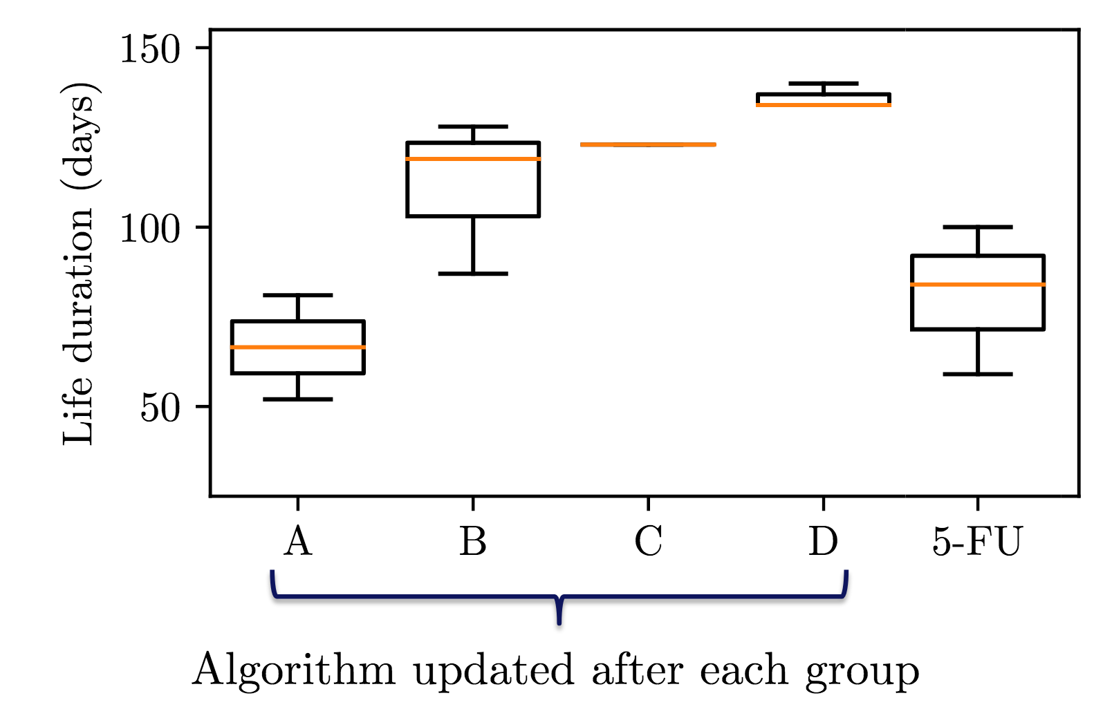 Fig 5.15. Experimental results of adaptive treatment (better than chemotherapy). Source: Audrey Durand
Moreover, each group had a slower tumour growth compared to the random experiment in phase 1 that resulted in exponential tumour growth. Using this adaptive treatment, mice lived longer with more controlled tumour growth that resulted in a better state space covering on larger tumour growth states.
A last interesting result shown in figure 5.16 was that the learned policy of treatment assignment, when we look at the last policy (most refined), we have Imiquimod (immunotherapy) all the time and gradually drops the 5FU (chemotherapy) which is consistent with researcher’s theory that the tumour could adapt to chemotherapy with time.
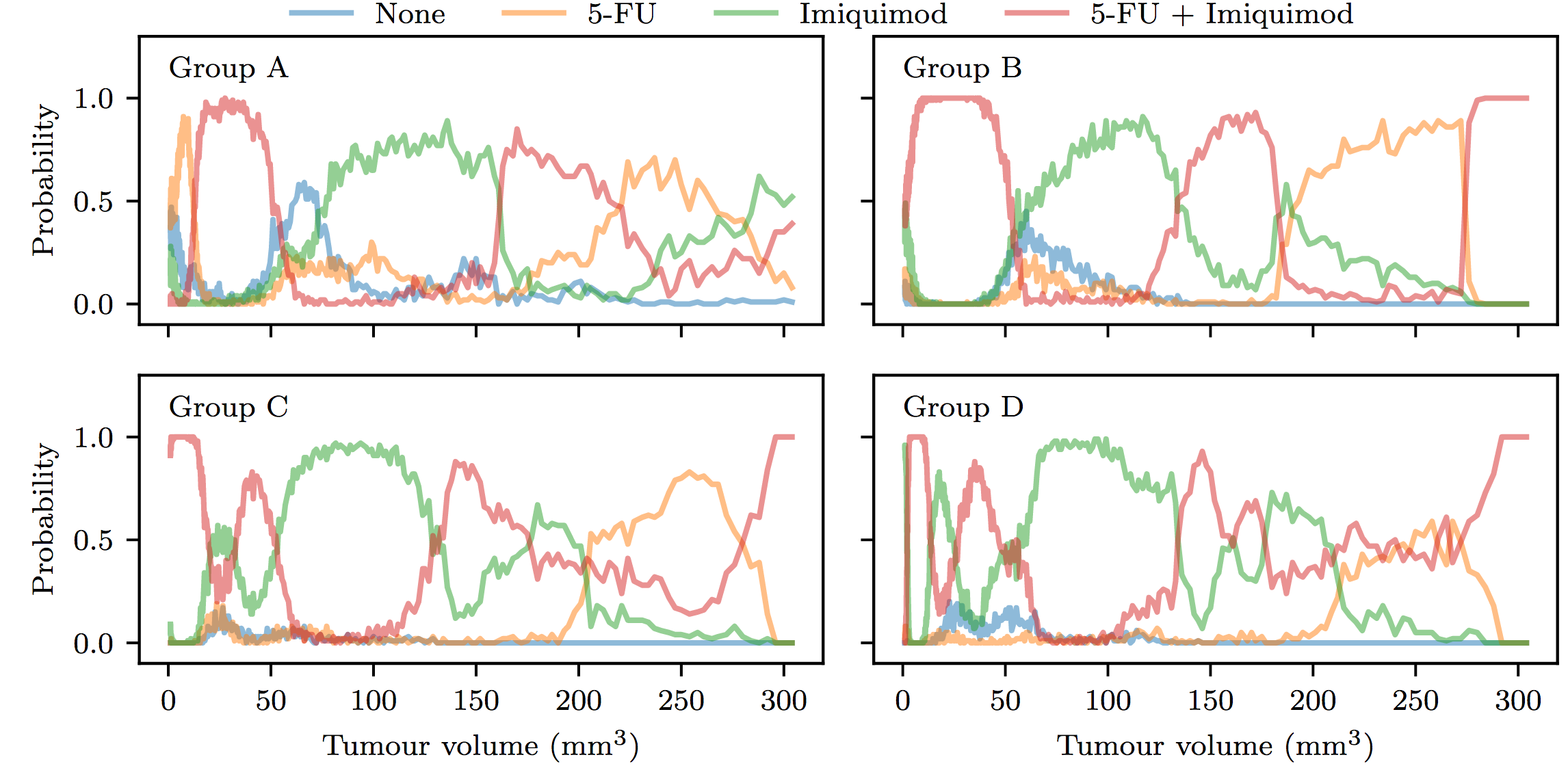 Fig 5.16. Learned treatment policies. Source: Audrey Durand
Conclusion
The researchers successfully applied structured and contextual bandits algorithm to a medical real life experiment and got good results. They had to drop some assumptions needed for the theory to work but showed that they retained good results in practice.