Sutton & Barto summary chap 10 - On-policy control
This post is part of the Sutton & Barto summary series.
- 10.1. Episodic Semi-gradient Control
- 10.2. Semi-gradient n-step Sarsa
- 10.3. Average rewards: a new problem setting for continuing tasks
- 10.4. Deprecating the Discounted Setting
- 10.5. Differential Semi-gradient n-step Sarsa
- 10.6. Summary
In Reinforcement Learning we talk a lot about prediction and control. Prediction refers to the prediction of how well a fixed policy performs, and control refers to the search of a better policy.
- After discussing the approximate case on-policy prediction problem in chapter 09, we now discuss the control problem in the same setting.
- It’s a “regular” control problem but now we have a parametric approximation of the action-value function $\hat{q}(s, a, \mathbf{w}) \approx q_*(s, a)$.
- We’ll see Semi-gradient Sarsa which is an extension of the semi-gradient TD(0) from last chapter, but with action-values
- Episodic extension is straightforward but continous is trickier
10.1. Episodic Semi-gradient Control
The approximate action-value function $\hat{q} \approx q_{\pi}$ is the parametrized function with weight vector $\mathbf{w}$. The general gradient-descent update for action-value prediction is:
- It looks a lot like the state value version presented in chapter 09
- $U_t$ is the target, for example $R_{t+1} + \gamma \hat{q}(S_{t+1}, A_{t+1}, \mathbf{w}_t)$ for one-step Sarsa, but it could be the full Monte-Carlo return or any of the n-step Sarsa returns
- With the one-step sarsa target, the method is called episodic semi-gradient one-step Sarsa
This forms the action-value prediction part, and for control we need to couple that to policy improvement and action selection techniques
- greedy action selection $A_t^* = \underset{a}{\mathrm{argmax}} \; \hat{q}(S_t, a, \mathbf{w}_t)$
- policy improvement: $\varepsilon$-greedy
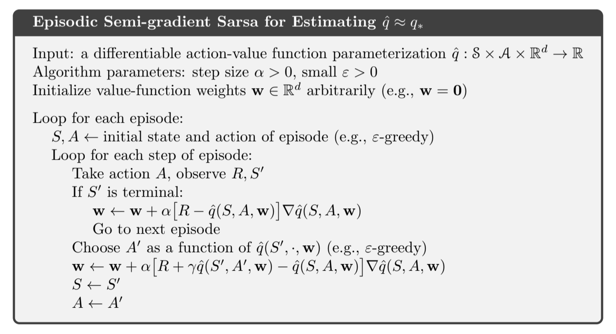
Fig 10.1. Episodic semi-gradient Sarsa
10.2. Semi-gradient n-step Sarsa
Use n-step return as the target ($U_t$) in the usual update:
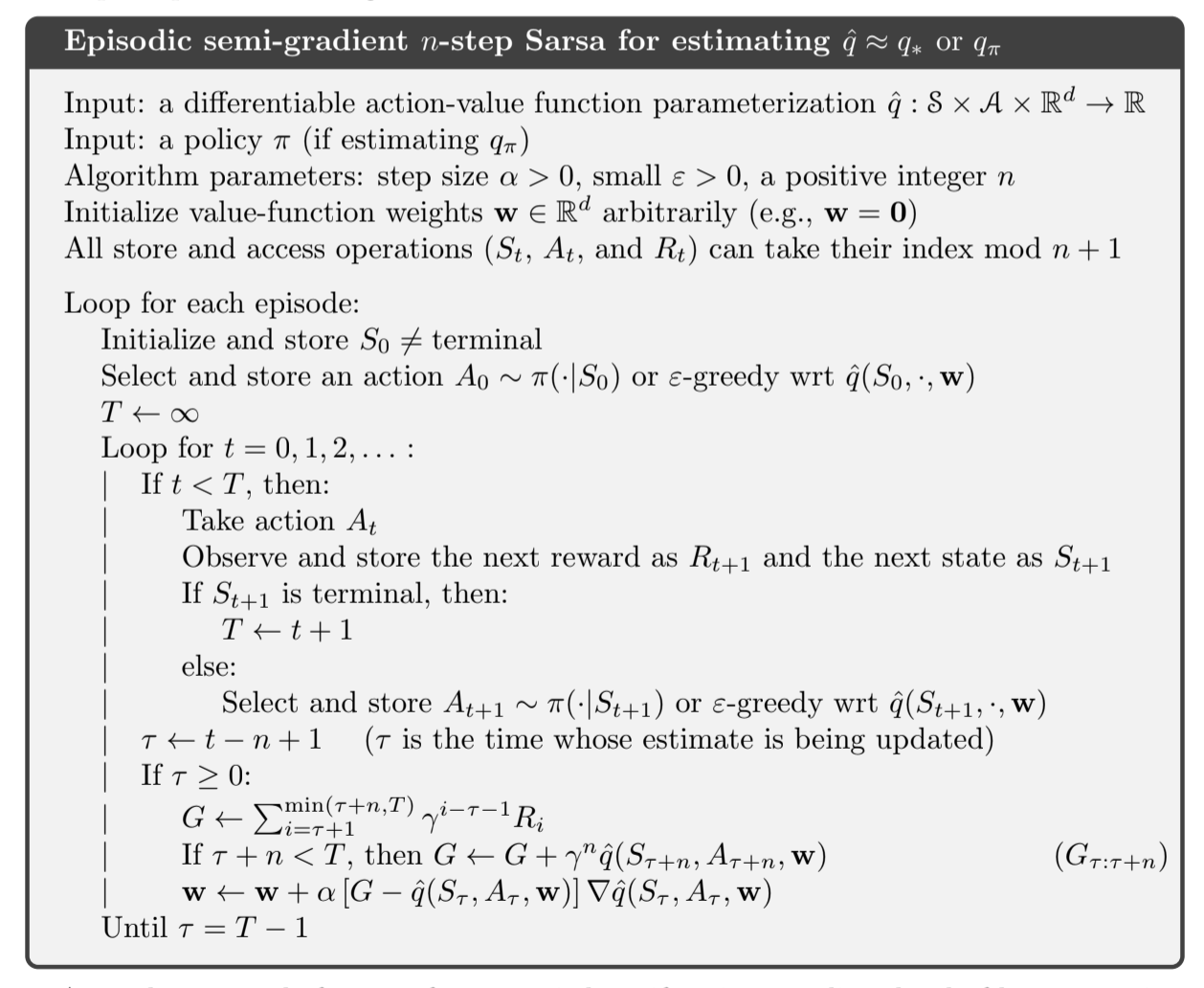
Fig 10.2. Episodic $n$-step semi-gradient Sarsa
10.3. Average rewards: a new problem setting for continuing tasks
We introduce a third classical setting for formulating the goal in MDPs:
- episodic setting
- discounted setting
- average reward setting
It applies to continuing problems with no start nor end. There is no discounting, and because the discounting setting is problematic with function approximation, this setting replaces it.
In the average reward setting, the quality of a policy $\pi$ is defined as the average rate of reward (short average reward) $r(\pi)$ while following that policy.
This works under the ergodicity assumption: $\mu_{\pi}$ is the steady-state distribution, and it exists for any $\pi$ independently of $S_0$. Aka starting state and early decisions have no effect in the limit.
- all policies that attain the maximal value of $r(\pi)$ are considered optimal
- the steady state distribution is the distribution under which when you select an action you end up in the same distribution. Formally, $\sum_s \mu_{\pi}(s) \sum_a \pi(a|s) p(s’|s, a) = \mu_{\pi}(s’)$
In the average-reward setting, returns are defined in terms of differences between rewards and average rewards (differential return):
The corresponding value functions are differential value functions (remove all $\gamma$ and replace rewards by the difference):
Differential forms of the TD error:
Where $\bar{R}_{t}$ is an estimate at time $t$ of the average reward $r(\pi)$
Sorry if it feels like I’m just throwing equations at you, these are just the differential value versions of useful quantities seen throughout the blogpost series, I feel it’s useful to have them all in one place.
With these alternative definitions, most of the algorithms already seen carry through the average-reward setting without change. For example, the average reward version of semi-gradient Sarsa is defined with the new version of the TD error:
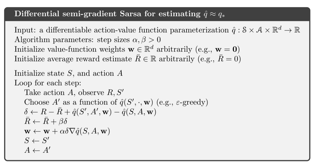
Fig 10.3. Differential Sarsa
10.4. Deprecating the Discounted Setting
- the discounted setting is useful for the tabular case where the return for each state can be separated and averaged
- in continuing tasks, we could measure the discounted return at each time step
- the average of the discounted rewards is proportional to the average reward, so the ordering of the policies don’t change, making discounting pretty useless
Proof
Idea: Symmetry argument. Each time step is the same as every other. With discounting each reward appears exactly once in the return. The $t$th reward will be undiscounted in the $t-1$st return, discounted once in the $t-2$th return, and so on. The weight of the $t$th reward is thus $1 + \gamma + \gamma^2 + … = 1 / (1 - \gamma)$. Because all states are the same, they are all weighted by this, and thus the average of the returns will be this weight times the average reward.
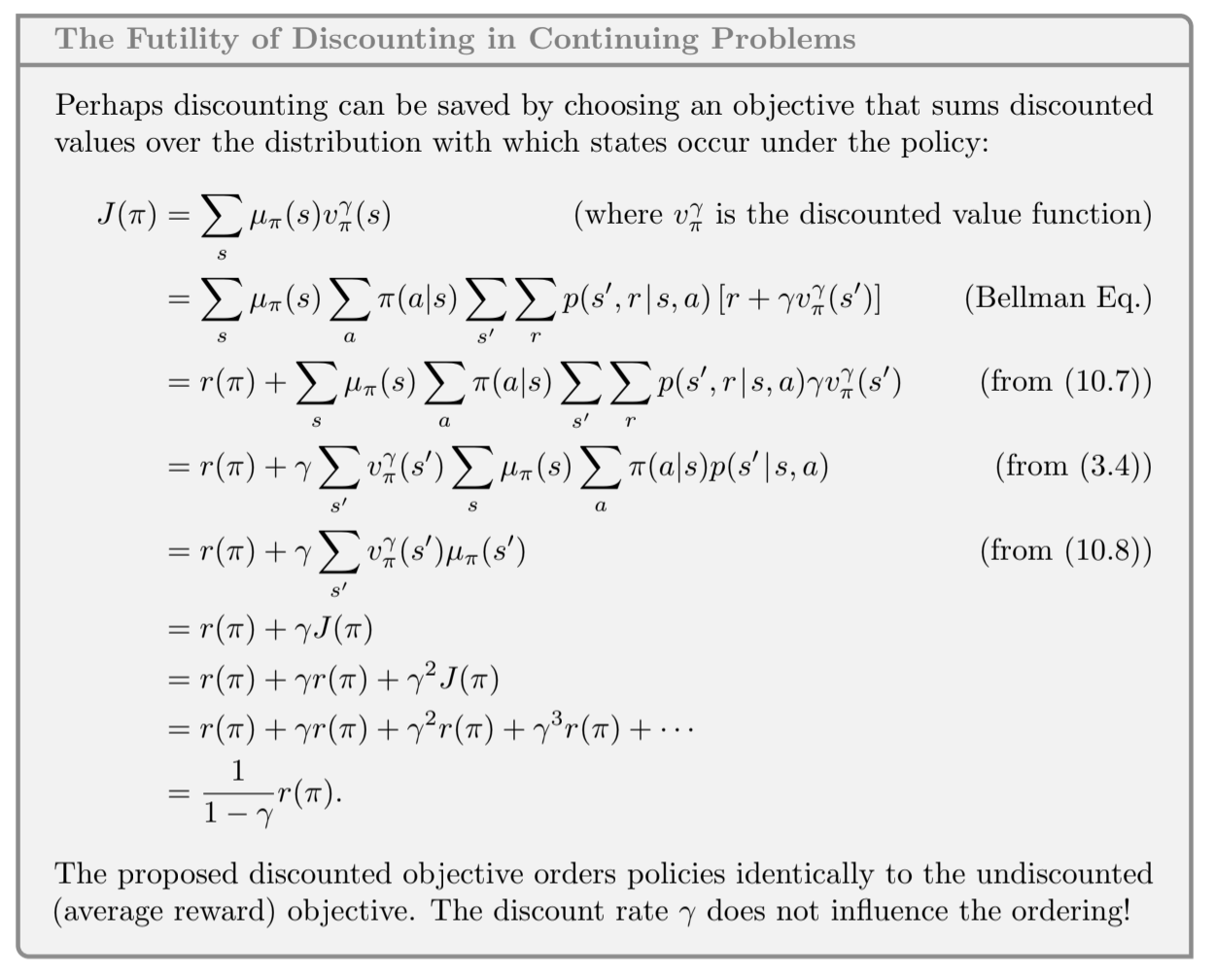
Fig 10.4. Proof that discounting is useless in the continuing setting
The root cause of the difficulties with discounting is that we lost the policy improvement theorem with function approximation. It is no longer true that if we change the policy to improve the discounted value of one state then we are guaranteed to have improved the overall policy. This lack of theoretical guarantees is an ongoing area of research.
10.5. Differential Semi-gradient n-step Sarsa
To generalize to n-step bootstrapping, we need an n-step version of the TD error. n-step return:
- $\bar{R}_{t}$ is an estimate of $r(\pi)$, $n \geq 1$ and $t + n < T$. If $t + n \geq T$, then we define $G_{t:t+n} = G_t$ as usual
- The n-step TD error is then:
And then we can apply the usual semi-gradient Sarsa update.
Algo:

Fig 10.5. Differential $n$-step Sarsa
10.6. Summary
- Extension of parametrized action-value functions and semi-gradient descent to control
- Average-reward setting replacing discounting for continuous case
- This new settings involves a differential version of everything