Sutton & Barto summary chap 08 - Planning and learning with tabular methods
This post is part of the Sutton & Barto summary series. This is our last post for the tabular case!
- 8.1. Models and Planning
- 8.2. Dyna: Integrated planning, acting, and learning
- 8.3. When the model is wrong
- 8.4. Prioritized sweeping
- 8.5. Expected vs sample update
- 8.6. Trajectory sampling
- 8.7. Real-time Dynamic Programming (RTDP)
- 8.8. Planning at Decision Time
- 8.9. Heuristic search
- 8.10. Rollout algorithms
- 8.11. Monte Carlo Tree Search (MCTS)
- 8.12. Summary of the Chapter
- 8.13. Summary of Part I: Dimensions
- model-based (Dynamic Programming, heuristic search) methods rely on planning
- model-free (Monte Carlo, Temporal Differences) methods rely on learning
Similarities:
- both revolve around the computation of value functions
- both look ahead of future events, compute a backed up value and use it as an update target for an approximate value function
In this chapter we explore how model-free and model-based approaches can be combined.
8.1. Models and Planning
models
A model is anything the agent can use to predict the environment’s behaviour.
- Given a state and an action, a model predicts the next state and the next reward.
- If the model is stochastic, we have several next possible states and rewards. The model can:
- Output the whole probability distribution over the next states and rewards: distribution models
- Produce only one of the possibility (the one with highest probability): sample models
- A model can be used to simulate the environment and produce simulated experience
planning
Planning refers to any computational process that takes a model as input and produces or improves a policy for interacting with the modeled environment.

We can distinguish two types of planning:
- state-space planning: search through the state space for an optimal policy. Actions cause transitions from state to state, and value functions are computed over states
- plan-space planning: search through the space of plans. Operators transform one plan into another (evolutionary methods, partial-order planning)
We focus on state-space planning, that share a common structure:

- All state-space planning methods involve computing value functions as key intermediate towards improving the policy
- they compute value functions by updates of backup operations applied to simulated experience
Ex: Dynamic Programming (DP) make sweeps through the space of states, generating for each the distribution of possible transitions. Each distribution is then used to compute a backed-up value (update target) and update the state’s estimated value.
- planning uses simulated experience generated by the model
- learning uses real experience generated by the environment
There are differences but in many cases a learning algorithm can be substituted for the key update step of a planning method, because they apply just as well to simulated experience. Let’s see an example with an algorithm we know: Q-learning.
random-sample one-step tabular Q-learning
Planning method based on Q-learning and random samples from a sample model:
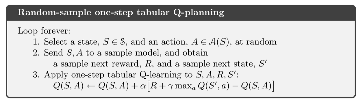
Fig 8.1. Planning Q-learning
In practice, we observe planning with very small steps seems to be the most efficient approach.
8.2. Dyna: Integrated planning, acting, and learning
When planning is done online, while interacting with the environment, a number of issues arise.
- new information may change the model (and thus the planning)
- how to divide the computing resources between decision making and model learning?
Dyna-Q: simple architecture integrating the major functions of an online planning agent
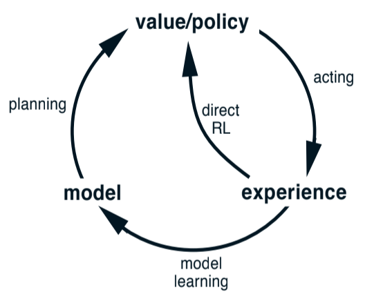
Fig 8.2. Dyna-Q interactions
What do we do with real experience:
- model-learning: improve the model (to make it more accurately match the environment)
- direct RL: improve the value functions and policy used in the reinforcement learning programs we know
- indirect RL: improve the value functions and policy via the model [that’s planning]
Both direct and indirect method have advantages and disadvantages:
- indirect methods often make fuller use of limited amount of experience
- direct methods are often simpler and not affected by bias in the design of the model
Dyna-Q
Dyna-Q includes all of the processes show in the diagram: planning, acting, direct RL and model-learning.
- the planning method is the random sample one-step tabular Q-learning shown above
- the direct RL method is one-step tabular Q-learning
- the model learning method is table based and assumes the environment is deterministic:
- After each transition $S_t, A_t \rightarrow S_{t+1}, R_{t+1}$, the model records in its table entry for $S_t, A_t$ the prediction that $S_{t+1}, R_{t+1}$ will follow.
- if the model is queries with a state-action pair it has seen before, it simply returns the last $S_{t+1}, R_{t+1}$ experienced
- during planning, the Q-learning algorithm samples only from state-actions the model has seen
Overall architecture of Dyna-Q agents:
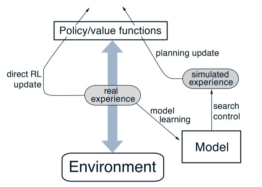
Fig 8.3. Dyna-Q agent architecture
- search control: process that selects starting states and actions from the simulated experiences
- planning is achieved by applying RL methods to simulated experience
Typically, as in Dyna-Q, the same algorithm is used for direct learning and for planning. Learning and planning are deeply integrated, differing only in the source of their experience.
Conceptually, planning, acting, direct RL and model-learning all occur in parallel. But for concreteness and implementation on a computer we specify the order:
- acting, model-learning and direct RL require little computation
- the remaining time in each step is devoted to planning which is inherently computationally intensive
Algorithm:
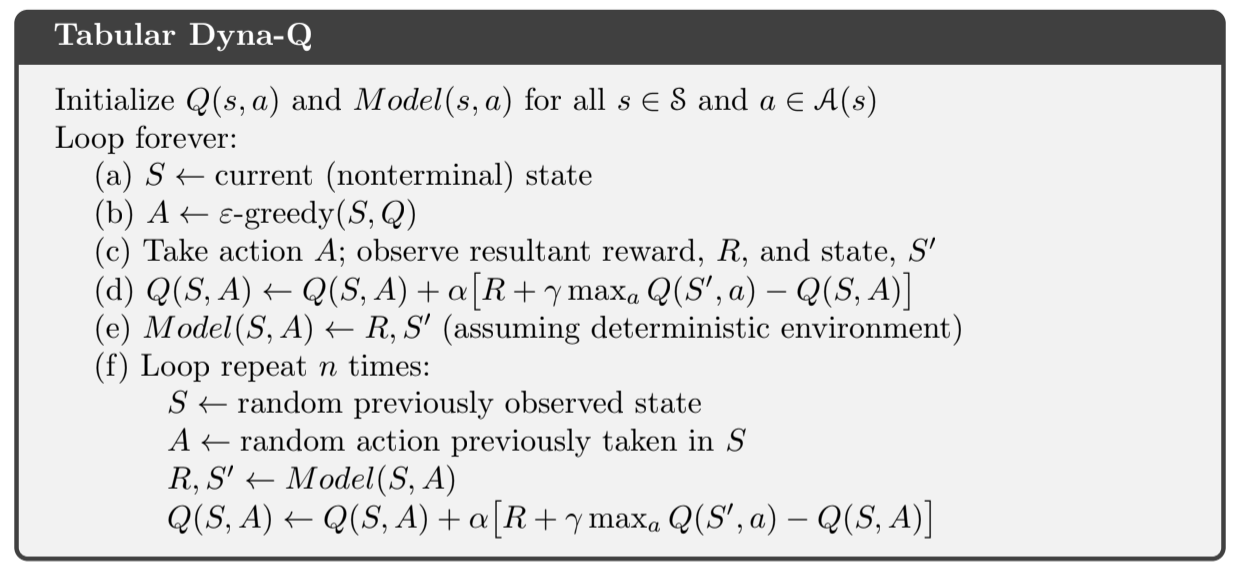
Fig 8.4. Dyna-Q algorithm
- $Model(s, a)$ denotes the content of the predicted $S_{t+1}$ and $R_{t+1}$ for $(s, a)$
- Direct RL, model-learning, planning are steps d, e, f respectively
- if e and f were omitted, the algorithm would be one-step tabular Q-learning
A simple maze example shows that adding the planning $n > 0$ element dramatically improves the agent behaviour.
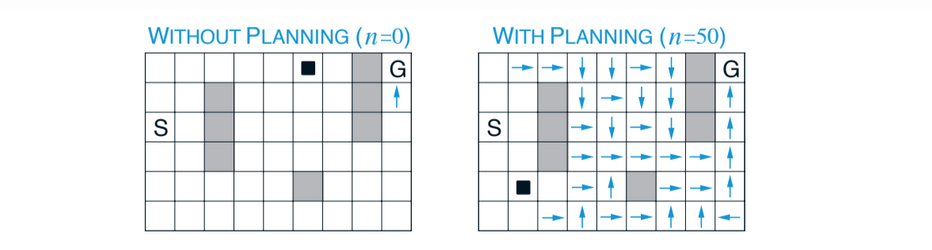
Fig 8.5. Dyna-Q planning example. The black square is the agent, the arrows denote the greedy action for the state (no arrow: all actions have equal value). These are the policies learned by a planning and a non-planning agent halfway through the second episode.
Intermixing planning and acting: make them both proceed as fast as they can:
- the agent is always reactive, responding with the latest sensory information
- planning is always done in the background
- model-learning is always done in the background too As new information is gained, the model is updated. As the model changes, the planning process will gradually compute a different way of behaving to match the newer model.
8.3. When the model is wrong
Models may be incorrect because:
- the environment is stochastic and only a limited amount of experience is available
- the model has learned using a function approximation that failed to generalize
- the environment has changed and new behaviour has not been observed yet
In some cases, following the suboptimal policy computed over a wrong model quickly leads to the discovery and correction of the modeling error, for example we will try to reach an expected reward that do not exist.
Example when the environment changes (the barrier moves a little):
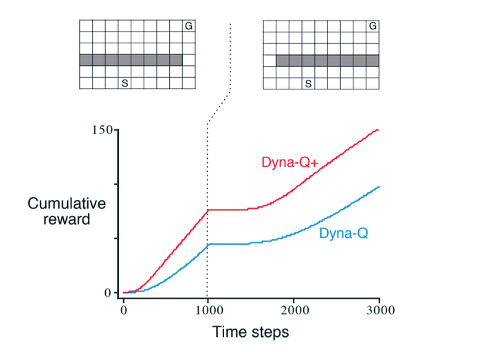
Fig 8.6. Blocking task. The left environment changes for the right environment after 1000 time steps. Dyna-Q+ is Dyna-Q with an exploration bonus.
Another example is when the environment changes to offer a better alternative without changing the availability of the learned path:
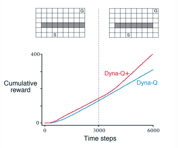
Fig 8.7. Shortcut task. The left environment changes for the right environment after 3000 time steps.
Exploration / exploitation tradeoff: we want the agent to explore to find changes in the environment but not so much that the performance is greatly degraded. Simple heuristics are often effective.
Dyna-Q+
Dyna-Q+ uses one such heuristic. This agent keeps track for each state-action pair of how many time steps have elapsed since it was last tried in a real interaction with the environment. A special bonus reward is added to simulated experience involving these actions. If the modeled reward for a transition is $r$, and the transition has not been tried for over $\tau$ time steps, then planning updates are done as if the transition produced a reward of $r + k \sqrt{\tau}$ for some small $k$. This encourages the agent to make some tests, which has a cost, but often is worth it.
8.4. Prioritized sweeping
So far for the dyna agents, simulated transitions are started in state-action pairs selected uniformly at random from all previously experienced state-action pairs. Uniform selection is usually not the best, and we’d better focus on particular state-action pairs.
For example at the beginning of the second episode in a normal maze, only the state-action pair leading to the goal has a positive value, and all other have a zero value. Updating all transitions would be very pointless, taking zero values to another zero value. We want to focus on state-actions around the state-action that led to the goal.
Backward-focusing of planning computations: in general, we want to work back not just from goal states but from any state whose value have changed.
As the frontier of useful updates propagates backward, it grows rapidly, producing many state-action pairs that could be usefully updated. But not all of them are equally useful. The value of some states have changed a lot, and the value of their predecessors are also likely to change a lot. It is then natural to prioritize them according to a measure of their urgency, and perform them in order of priority.
This is prioritized sweeping. A queue is maintained for every state-action pair whose value would change if updated, prioritized by the size of the change.
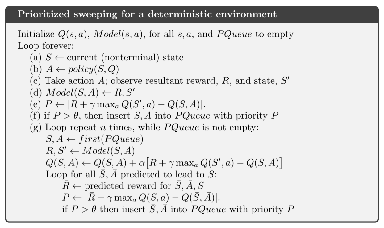
Fig 8.8. Prioritized sweeping algorithm
Prioritized sweeping has been found to dramatically increase the speed of convergence.
What about stochastic environments
The model is maintained by keeping counts of the number of times each state-action pair has been experienced and what their next states were. We can update each state-action pair not with a sample update but with an expected update, taking into account the possibilities of the next states and their probability of occurring.
Using expected updates can waste a lot of computation on low-probability transitions. Often using samples help converge faster despite the added variance. Sample updates can be better because they break the overall backing-up computation into smaller pieces (individual transitions) which enables them to be more focused on the pieces that would have the greater impact.
Summary
We have suggested in this chapter that all kinds of state-space planning can be viewed as sequences of value updates, varying only in:
- the type of update, expected or sample, large or small,
- the order in which the updates are done
We have focused on backward focusing, but this is only one strategy. Another could be to focus on states according to how easy they can be reached from the states that are visited frequently under the current policy, which can be called forward focusing.
8.5. Expected vs sample update
The examples of the previous sections give an idea of how planning and learning can be combined. Now we’ll focus on each of the components, starting with expected vs sample update.
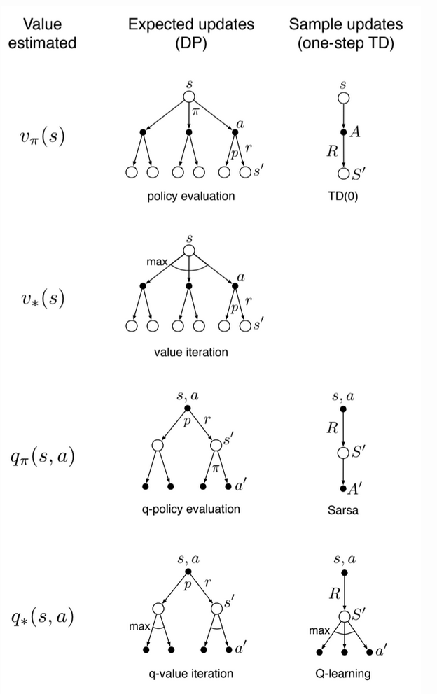
Fig 8.9. Backup diagrams for one-step updates
We have considered many value-function updates. If we focus on one-step upates, they vary along 3 dimensions:
- Update state value or action values
- Estimate the value of the optimal policy or any given policy
- The updates are expected updates (consider all possible events) or sample updates (consider a sample of what might happen)
These 3 binary dimensions give rise to 8 cases, seven of which are specific algorithms, shown on the figure on the right.
(the eighth case doesn’t seem to yield any meaningful update)
Any of these one-step method can be used in planning methods.
- The Dyna-Q discussed before use $q_*$ sample updates but could use $q_*$ expected update or $q_{\pi}$ updates.
- The Dyna-AC system uses $v_{\pi}$ sample updates with a learning policy structure
- For stochastic problems, prioritized sweeping is always done using one of the expected updates
When we don’t have the environment model, we can’t do an expected model so we use a sample. But are expected update better than sample updates when available?
- they yield a better estimate because they are uncorrupted by sampling error
- but they require more computation
Computational requirements
For $q_*$ approximation in this setup:
- discrete states and actions
- table-lookup representation of the approximate value function Q
- a model in the form of estimated dynamics $\hat{p}(s’, r|s, a)$
The expected update is:
The sampl update is the Q-learning like update:
The difference between these expected and sample updates is significant to the extent that the environment is stochastic. Many possible next states = many computation for the expected update.
For a particular set $(s, a)$, let $b$ be the branching factor, aka the number of possible next states. Then an expected update of this pair requires roughly $b$ times as much computation as a sample update.
Given a unit of computational effort, is it better devoted to a few expected updates or to $b$ times as many sample updates?
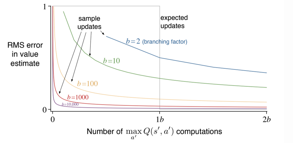
Fig 8.10. Comparison of the efficiency of expected and sample updates
Figure 8.10 shows the estimation error a a function of computation time for various branching factors. All successors are considered equally likely and the error in the initial estimate is 1.
For moderately large b the error falls dramatically with a tiny fraction of b updates. For these cases, many state-action pairs could have their values improved dramatically in the same time that a single action-pair could undergo an expected update.
By causing estimates to be more accurate sooner, sample updates will have an advantage that the values backed up from the succesor states will be more accurate.
TL;DR: sample updates are better to expected updates on problems with a large branching factor and too many states
8.6. Trajectory sampling
Here we compare 2 ways of distributing updates:
- exhaustive sweep: classical approach from DP: perform sweeps through the entire state space, updating each state once per sweep
- sample from the state space according to some distribution
- uniform sample: Dyna-Q
- on-policy distribution (interact with the model following the current policy). Sample state transitions and rewards are given by the model, and sample actions are given by the current policy. We simulate explicit individual trajectories and perform update at the state encountered along the way -> trajectory sampling
Is the on-policy distribution a good one?
- it causes vast, uninteresting parts of the space to be ignored
- could be bad because we update the same parts over and over
In the book there is a series of experiments showing that on-policy sampling result in faster planning initially and a little bit retarded (sic) in the long run. Focusing on the on-policy distribution may hurt in the long run because the commonly occurring states all already have their correct value. Sampling them is useless. This is why exhaustive sampling is better in the long run, at least for small problems. For large problems, the on-policy sampling is more efficient.
8.7. Real-time Dynamic Programming (RTDP)
RTDP is an on-policy trajectory-sampling version of the value-iteration algorithm of DP. It is closely related to full-sweep policy iteration so we illustrate some advantages that on-policy trajectory sampling can have.
RTDP updates the values of states visited in actual or simulated trajectories by means of expected tabular value-iteration updates.
RTDP is an example of an asynchronous DP algorithm. Asynchronous algorithms do not do full sweeps, they update state values in any order, using whatever value of other states happen to be available. In RTDP, th update order is dictated by the order states are visited in real or simulated trajectories.
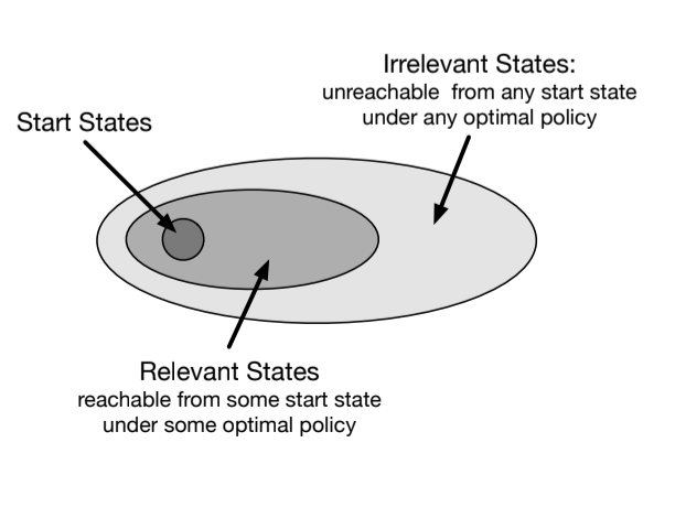
Fig 8.11. Classification of states
Evaluation
- trajectories start from a designated set of start states
- we have a prediction problem for a given policy
- on-policy trajectory sampling allows to focus on useful states
Improvement
For Control, the goal is to find an optimal policy instead of evaluating a given policy, there might be states that cannot be reached by any of the optimal policies from any of the start states, so there is no need to specify optimal actions for those irrelevant states. We in fact only need an optimal partial policy.
Finding such an optimal partial policy can require visiting all state-action pairs, even those turning out to be irrelevant in the end. It is generally not possible to stop updating any state if convergence to an optimal policy is important.
For certain types of problems under certain conditions, RTDP is guaranteed to fin a policy that is is optimal on the relevant states without visiting every state infinitely often, or even without visiting some states at all.
- The task must be an undiscounted episodic task for MDP with absorbing goal state that generate zero reward.
At every step or a real or simulated trajectory, RTDP selects a greedy action and applies the expected value-iteration update operation to the current state. It can also update other states, like those visited in a limited-horizon look-ahead search from the current state.
More conditions for guarantee of optimal convergence:
- the initial value of every goal state is 0
- there exists at least one policy that guarantees a goal state will be reached from any start state
- all rewards from transitions from non-goal states are strictly negative
- the initial values are $\geq$ to optimal values
Proof: Barto, Bradtke and Singh 1995
Tasks having these properties are examples of stochastic optimal path problems, which are usually stated in term of cost minimization instead of reward maximization, but we can just maximize the negative returns.
Results of RTDP on the racing car problem:
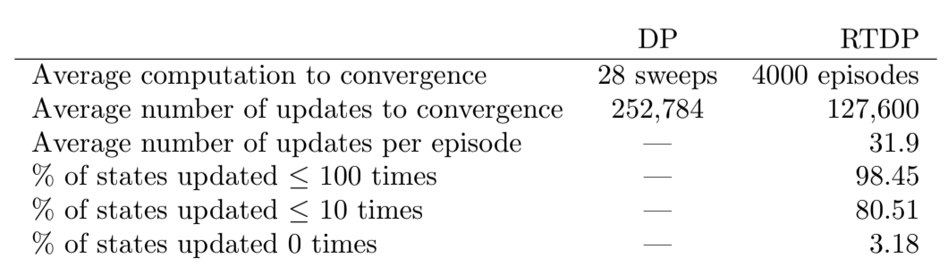
Fig 8.12. RTDP car racing results
RTDP only required half of the updates that DP did. This is the result of RTDP’s on-policy trajectory sampling.
As the value function approaches $v_*$, the policy used by the agent to generate trajectories approaches an optimal policy because it is always greedy wrt the current value function. This is unlike traditional value iteration, where it terminates when the value function changes by a tiny amount in a sweep. It is possible that policies that are greedy wrt the latest value function were optimal long before value iteration terminates! Checking the emergence of an optimal policy before value iteration converges is not a part of conventional DP and requires way more computation.
In the example, the DP method ha an optimal policy emerged at 136 725 value iteration updates, les that the 252 784 updates DP needed but still more than the 127 600 updates of RTDP.
8.8. Planning at Decision Time
Planning can be used in two ways.
- bakcground planning: so far (Dyna, DP), we use planning to gradually improve a policy or value function on the basis of simulated experience from a model. We then select actions by comparing the current state’s action values. Well before an action is selected for any current state $S_t$, planning has played a part in improving the way to select the action for many states, including $S_t$. Planning here is not focused on the current state.
- decision-time planning: begin and complete planning after encountering each state $S_t$, to produce a single action $A_t$. Dummy example: planning when only state-values are available, so at each state we select an action based on the values of model-predicted next states for each action. We can also look much deeper than one step ahead. Here planning focuses on a particular state.
decision-time planning
Even when planning is done at decision time, we can still view it as proceeding from simulated experience to updates and values, and ultimately to a policy. It’s just that now the values and policy are specific to the current state. Those values and policies are typically discarded right after being used to select the current action.
In general we may want to do a bit of both:
- focus planning on th current state
- and store the results of planning so as to help when we return to the same state after
Decision-time planning is best when fast responses are not required. If low latency action selection is the priority, we’re better off doing planning in the background to compute a policy that can be rapidly used.
8.9. Heuristic search
The classical state-space plannng methods are decision-time planning methods collectively known as heuristic search. In heuristic search, for each state encountered, a large tree of possible continuations is considered. The approximate value function is applied to the leaf nodes and then backed up toward the current state at the root, then the best is chosen as the current action, and all other backed-up values are discarded.
Heuristic search can be viewed as an extension of the idea of a greedy policy beyond a single step, to obtain better action selections. If the search is of sufficient depth $k$ such that $\gamma^k$ is very small, then the actions withh be correspondingly near optimal. The tradeoff here is that deeper search leads to more computation.
Much of the effectiveness of heuristic search is due to its search tree being tightly focused on the states and actions that might immediately follow the current state. This great focusing of memory and computational resources on the current decision is presumably the reason why heuristic search can be so effective.
The distribution of updates can be altered in similar ways to focus on the current state and its likely successors. As a limiting case we might use exactly the methods of heuristic search to construct a search tree, and then perform the individual, one-step updates from bottom up:
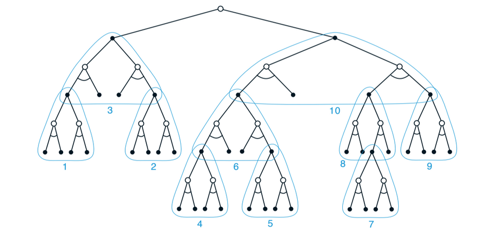
Fig 8.13. Heuristic search as a sequence of one-step updates (in blue), backing up values from leaf to root. The ordering here is selective depth-first search.
8.10. Rollout algorithms
Rollout algotihms are decision-time planning algorithms based on Monte Carlo control applied to simulated trajectories that all begin at the current environment state. They estimate action values for a given policy by averaging the returns of many simulated trajectories that start with each possible action and then follow the given policy. When the action-value estimates are accurate enough, the best one is executed and the process starts anew from the resulting next state.
Unlike MC algorithm, the goal here is not to estimate a complete optimal action-value function. Instead, we only care about the current state and one given policy, called the rollout policy. The aim of a rollout algorithm is to improve upon the rollout policy, not to find an optimal policy.
The computation time needed by a rollout algorithm depends on many things, including the number of actions that have to be evaluated for each decision, and the number of time steps in the simulated trajectories. It can be demanding but:
- it is possible to run many trials in parallel on separate processes because Monte Carlo trials are independent of one another
- we can truncate the trajectories short of complete episoeds and correct the truncated returns by the means of a stored evaluation function
- monitor the Monte Carlo simulations and prune away actions that are unlikely to be the best
Rollout algorithms are not considered learning algorithms since they do not maintain long term memory of values or policies, but they still use reinforcement learning techniques (Monte Carlo) and take advantage of the policy improvement property by acting greedily wrt the estimated action values.
8.11. Monte Carlo Tree Search (MCTS)
Recent example of decision-time planning. It is basically a rollout algorithm, but enhanced with a means of accumulating value estimates from the Monte Carlo simulations, in order to successively direct simulations towards more highly-rewarding trajectories. It has been used in AlphaGo.
MCTS is executed after encountering each new state to select the action. Each execution is an iterative process that simulates many trajectories starting from the current state and running to a terminal state (or until discounting makes any further reward negligible). The core idea of MCTS is to successively focus multiple simulations starting at the current state by extending the initial portions of trajectories that have received high evaluations from earlier simulations.
The actions in the simulated trajectories are generated using a simple policy, also called a rollout policy. As in any tabular MC method, the value of a state-action pair is estimated as the average of the (simulated) returns from that pair. MC value estimates are maintained only for the subset of state-action pairs that are most likely to be reached in a few steps:
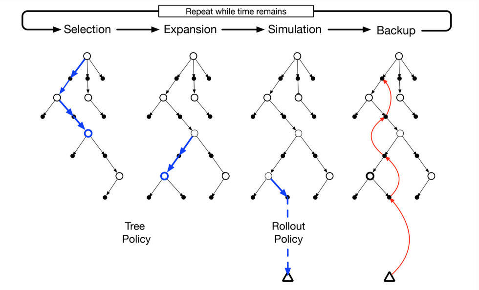
Fig 8.14. MCTS
MCTS incrementally extends the tree by adding promising nodes based on the result of simulated trajectories. Any simulated trajectory will pass through the tree and exit at some leaf node. Outside the tree and at leaf nodes the rollout policy is used to pick actions, but inside the tree we use the tree policy that balances exploration and exploitation (like an $\varepsilon$-greedy policy).
In more detail, each iteration of a basic MCTS consists of the following four steps:
- Selection. Starting at the root node, a tree policy based on the action value attached to the edges of the tree traverses the tree to select a leaf node.
- Expansion. On some iterations, the tree is expanded from the selected leaf node by adding one or more child nodes reached from the selected node via unexplored actions
- Simulation. From the selected node or its newly added children, simulation of a complete episode is run with actions selected first by the tree policy and beyond the tree by the rollout policy.
- Backup. The return generated by the simulated episode is backed up to update or initialize the action values attached to the edge of the tree traversed by the tree policy in this iteration of MCTS. No values are saved for the states and actions visited by the rollout policy beyond the tree. In figure 8.10 is shown a backup from the terminal state of the simulated trajectory directly to the state-action node in the tree where the rollout policy began (in general the entire return over the simulated trajectory is backed up to this state-action node)
MCTS continues executing these 4 steps, starting ach time at the tree’s root node, until no more time is left. Then, finally, an action from the root node (which still represent the current state of the environment) is selected (maybe the action having the largest action value, or the highest visit count). After the action is selected, the environment transitions into a new state and MCTS is run again, often starting with a tree that contains the relevant nodes from the tree constructed by the previous execution. All the remaining nodes are discarded along with their action values.
summary
- MCTS is a decision-time planning algorithm based on Monte Carlo control applied to simulations that start from the root state
- it saves action-value estimates attached to the tree edges and updates then using sample updates (this focuses trajectories)
- MCTS expands its tree, so it effectively grows a lookup table to store a partial action-value function
MCTS thus avoids the problem of globally approximating an action-value function while it retains the benefit of using past experience to guide exploration.
8.12. Summary of the Chapter
Planning requires a model of the environment.
- A distribution model consists of the probabilities of next states and rewards for possible actions. DP requires a distribution model to be able to use expected updates, which involves computing an expectation over all possible states and rewards.
- A sample model is needed to simulate environment interation and use sample updates.
There is a close relationship between planning optimal behaviour and learning optimal behaviour:
- both involve estimating the same value functions
- both naturally update the estimates incrementally, in a long series of backing-up operations
- any of the learning methods can be converted into planning methods simply by running them over simulated data
Dimensions
- size of the update: The smaller the update, the more incremental the planning methods can be. Small updates: one-step sample updates like Dyna
- distribution of updates (of the focus of the search):
- Prioritized sweeping focuses backward on the predecessors of interesting states
- On-policy trajectory sampling focuses on states that are likely
Planning can also focus forward from pertinent states, and the most important form of this is when planning is done at decision time. Rollout algorithms and MCTS benefit from online, incremental, sample-based value estimation and policy improvement.
8.13. Summary of Part I: Dimensions
Each idea presented in this part can be viewed as a dimension along which methods vary. The set of the dimensions spans a large space of possibe methods.
All the methods so far have three key ideas in common:
- they all seek to estomate value functions
- they all operate by backing up values along actual or possible state trajectories
- they all follow GPI, meaning that they maintain an approximate value function and an approximate policy, and they continually improve each based on the other.
main dimensions
Two of the most important dimensions are shown on figure 8.15.
- Whether we use sample updates based on a sample trajectory or an expected update based on a distribution of possible trajectories
- Depth of updates
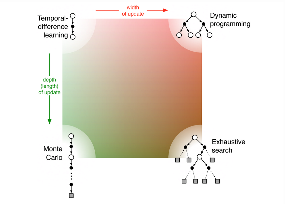
Fig 8.15. Main dimensions: depth and width. The space of RL methods spans all this!
other dimensions
- binary distinction between off-policy and on-policy methods
- definition of return: is the task episodic, discounted or undiscounted?
- action values vs state values vs afterstate values
- action selection / exploration: we have considered simple ways to do this: $\varepsilon$-greedy, optimistic init, softmax and upper confidence bound (UCB)
- synchronous vs asynchronous: are the updates for all states performed simultaneously or one by one in some order?
- real vs simulated
- location of updates: what states should be updated? Model free can only choose among encountered stats but model-based methods can choose arbitrarily.
- timing of updates: should updates be done as part of selecting actions or only afterwards?
- memory of updates: how long should updated values be retained?