Sutton & Barto summary chap 07 - N-step bootstrapping

This post is part of the Sutton & Barto summary series.

• 7.1. $n$-step Prediction
  • Targets
  • Error-reduction property
• 7.2. $n$-step Sarsa
  • Expected Sarsa
• 7.3. $n$-step Off policy learning by importance sampling
• 7.4. Per-decision Off-policy methods with Control Variates
  • For action values
• 7.5. Off-policy without importance sampling: The n-step backup tree algorithm
• 7.6. A Unifying algorithm: $n$-step $Q(\sigma)$
• 7.7. Summary

• Unify the Monte Carlo (MC) and one-step Temporal Difference (TD) methods
• n-step TD methods generalize both by spanning a spectrum with MC on one end and one-step TD at the other
• n-step methods enable bootstrapping over multiple time steps, which is nice because using only one time-step can reduce the power of our algorithms

7.1. $n$-step Prediction

Consider estimating $v_{\pi}$ from sample episodes generated using $\pi$.

• Monte Carlo methods perform an update for each visited state based on the entire sequence of rewards from that state until the end of the episode
• one-step TD methods update is based on the next reward only
• n-step: in-between

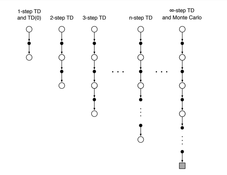
Fig 7.1. Backup diagrams for $n$-step methods, to show the spectrum between one-step TD and MC

Still TD: we bootstrap because we change an earlier estimate based on on how it differs from a later estimate (only that the later estimate is now n step later)

Targets

notation: $G_t^{(n)} = G_{t:t+n}$, the return from time step $t$ to $t+n$.

$$\begin{align} n = 1 & \quad (TD) \quad & G_t^{(1)} = R_{t+1} + \gamma V_t(S_{t+1}) \label{eq:7.1}\tag{7.1}\\ n = 2 & & G_t^{(2)} = R_{t+1} + \gamma R_{t+2} + \gamma^2 V_{t+1}(S_{t+2})\\ \vdots & & \vdots\\ n = \infty & \quad (MC) \quad & G_t^{(\infty)} = R_{t+1} + \gamma R_{t+2} + ... + \gamma^{T-1} R_T \label{eq:7.2}\tag{7.2} \end{align}$$

• In MC the target is the return
• In one-step TD the target is the one-step return, that is the first reward plus the discounted estimated value of the next state
• $V_t: \mathcal{S} \rightarrow \mathbb{R}$ is the estimate at time $t$ of $v_{\pi}$

n-step target:

$$G_t^{(n)} = R_{t+1} + \gamma R_{t+2} + ... + \gamma^{n-1} R_{t+n} + \gamma^n V_{t+n-1}(S_{t+n}) \label{eq:7.3}\tag{7.3}$$

• All n-step returns can be considered approximations of the full return, truncated after n steps and then corrected for the remaining steps by $V_{t+n-1}(S_{t+n})$
• n-steps return for $n > 1$ involve future rewards that are not available from the transition $t \rightarrow t + 1$. We’ll see eligibility traces (chapter 12) for an online method not involving future rewards.
• Plugging this into the state-value learning:

$$V_{t+n}(S_t) \doteq V_{t+n-1}(S_t) + \alpha[G_t^{(n)} - V_{t+n-1}(S_t)] \label{eq:7.4}\tag{7.4}$$

• no changes are made during the first n-1 steps of each episodes. to make up for that, an equal number of updates are made after the termination of the episode, before starting the next.

Algorithm:

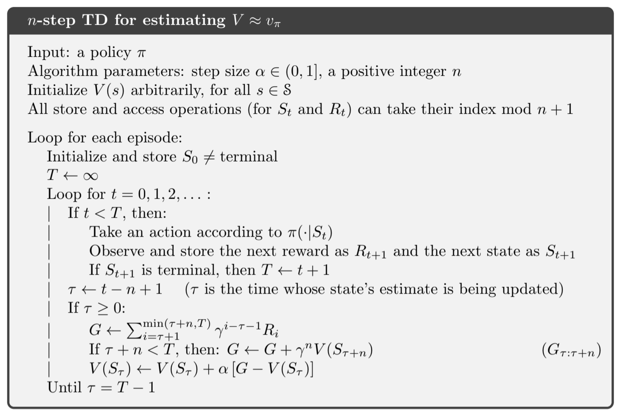
Fig 7.2. $n$-step TD algorithm

Error-reduction property

The n-step return uses the value function $V_{t+n-1}$ to correct for the missing rewards beyond $R_{t+n}$. An important property of the n-step returns is that their expectation is guaranteed to be a better estimate of $v_{\pi}$ than $V_{t+n-1}$ is, in a worst-state sense. The worst error of the expected n-step return is guaranteed to be less than or equal to $\gamma^n$ times the worst error under $V_{t+n-1}$.

$$\underset{s}{\mathrm{max}} \; | \mathbb{E}_{\pi} [G_t^{(n)} | S_t = s] - v_{\pi}(s) | \leq \gamma^n \underset{s}{\mathrm{max}} \; | V_{t+n-1}(s) - v_{\pi}(s)| \label{eq:7.5}\tag{7.5}$$

This is called the error reduction property. We can use this to show that all n-steps methods converge to the correct predictions under appropriate technical conditions.

We use this type of graph to show the effect of n:

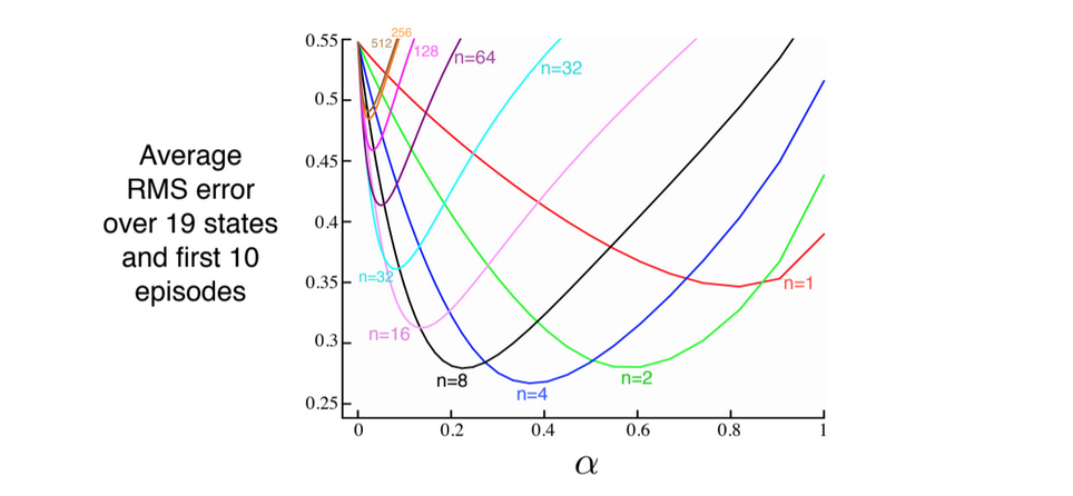
Fig 7.3. Performance of $n$-step TD methods as a function of $\alpha$ (learning rate)

7.2. $n$-step Sarsa

• Use n-step not just for prediction but also for control
• Switch states for state-action pairs and use a $\varepsilon$-greedy policy
• The backup diagrams for n-step Sarsa are like those of n-step TD except that the Sarsa ones start and end in a state-action node
• We redefine the n-step return in terms of estimated action-values instead of state-values:

$$G_{t:t+n} = R_{t+1} + \gamma R_{T+2} + ... + \gamma^{n-1} R_{t+n} + \gamma^n Q_{t+n-1}(S_{t+n}, A_{t+n}) \label{eq:7.6}\tag{7.6}$$

• And plug that into our GPI update:

$$Q_{t+n}(S_t, A_t) \gets Q_{t+n-1}(S_t, A_t) + \alpha \big(G_{t:t+n} - Q_{t+n-1}(S_t, A_t)\big) \label{eq:7.7}\tag{7.7}$$

The values of all other states remain unchanged, $Q_{t+n}(s, a) = Q_{t+n-1}(s, a)$ for $s \neq S_t$ or $a \neq A_t$.

Algorithm

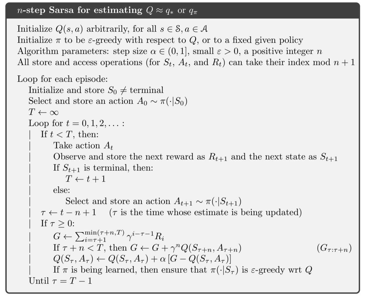
Fig 7.4. $n$-step Sarsa

Backup diagrams

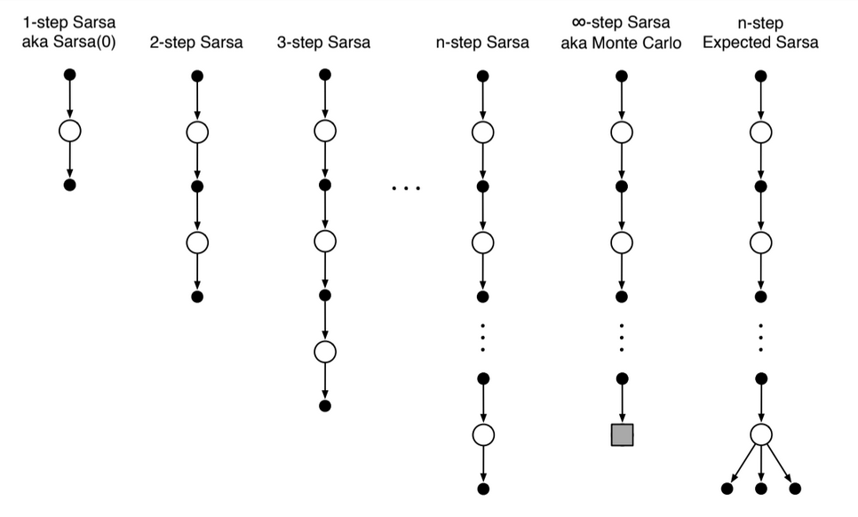
Fig 7.5. $n$-step Sarsa backup diagram

Expected Sarsa

What about n-step version of expected sarsa? The backup diagram consists of a linear string of sample actions and states and the last element is a branch over all action possibilities, weighted by their probability of occurring under $\pi$. The n-step return is here defined by:

$$G_{t:t+n} = R_{t+1} + \gamma R_{T+2} + ... + \gamma^{n-1} R_{t+n} + \gamma^n \bar{V}_{t+n-1}(S_{t+n}, A_{t+n}) \label{eq:7.8}\tag{7.8}$$

Where $\bar{V}_{t}(s)$ is the expected approximate value of state s, using the estimated action values and the policy:

$$\bar{V}_{t}(s) \doteq \sum_a \pi(a|s) Q_t(s, a) \label{eq:7.9}\tag{7.9}$$

• Expected approximate values are important!
• If s is terminal then its approximated value is defined to be $0$

7.3. $n$-step Off policy learning by importance sampling

• In order to use the data from the behaviour policy $b$, we must take into account the relative probability of taking the actions that were taken.
• In n-step methods the returns are constructed over n steps so we’re interested in the relative probability of just these n actions.

For example to make a simple version of n-step TD, we can weight the update for time $t$ (made at time $t+n$) by the importance-sampling ratio:

$$\rho_{t:h} = \prod_{k=t}^{min(h, T-1)} \frac{\pi(A_k\|S_k)}{b(A_k\|S_k)} \label{eq:7.10}\tag{7.10}$$

If we plug this into our update we get:

$V_{t+n}(S_t) \gets V_{t+n-1}(S_t) + \alpha$$\rho_{t:t+n-1}$$\big(G_{t:t+n} - V_{t+n-1}(S_t)\big)$

Note that if the two policies are actually the same (on-policy), the importance sampling ratio is always 1 and we have our previous update.

Similarly, the n-step Sarsa update can be extended for the off-policy method:

$Q_{t+n}(S_t, A_t) \gets Q_{t+n-1}(S_t, A_t) + \alpha$$\rho_{t+1:t+n-1}$$\big(G_{t:t+n} - Q_{t+n-1}(S_t, A_t)\big)$

Note that the importance sampling ratio here starts one step later than from n-step TD because we are updating a state-action pair (we know that we have selected the action so we need importance sampling only for the subsequent actions).

Algorithm:

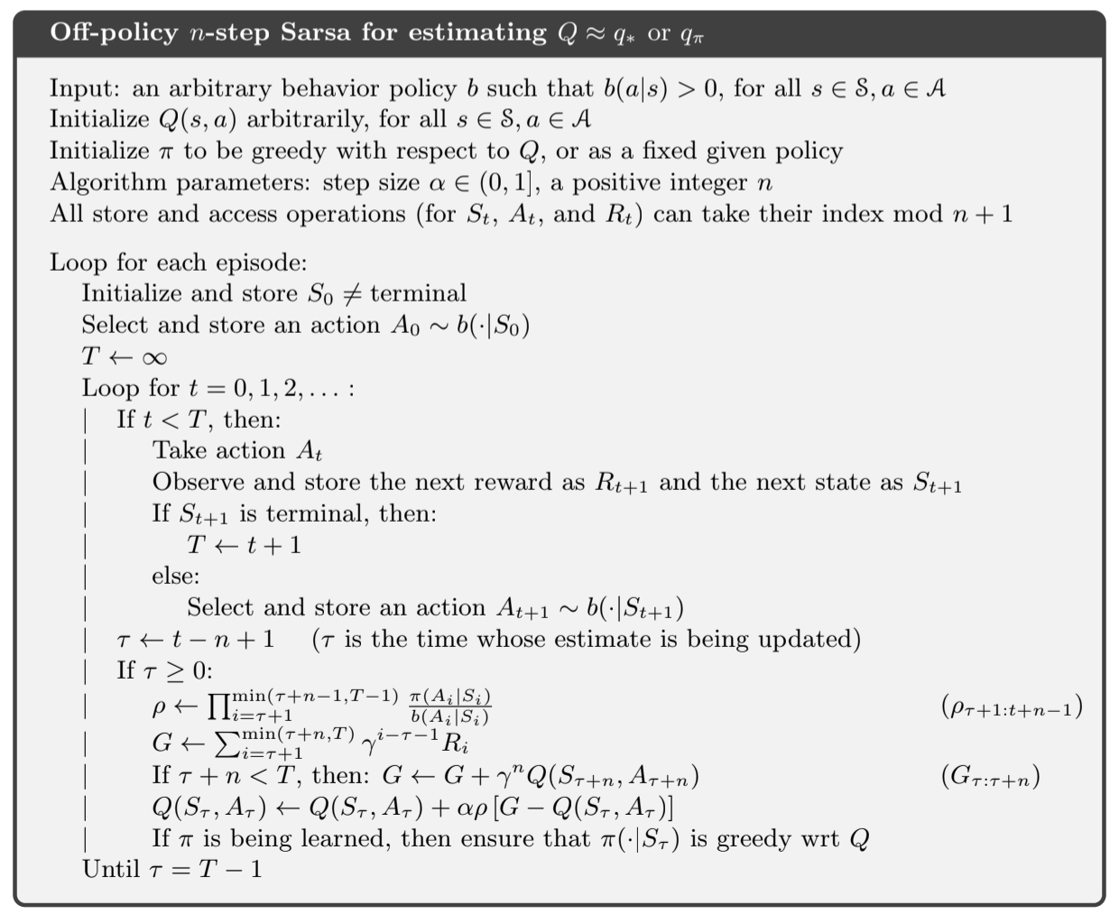
Fig 7.6. $n$-step Sarsa off-policy algorithm

The off-policy version for expected Sarsa would be the same except that the importance sampling ratio would use $\rho_{t+1:t+n-2}$ instead of $\rho_{t+1:t+n-1}$ because all possible actions are taken into account in the last state, the one actually taken has no effect and does not need to be corrected for.

7.4. Per-decision Off-policy methods with Control Variates

The multi-step off-policy method presented in 7.3 is conceptually clear but not very efficient. What about per-decision sampling?

1. the n-step return can be written recursively. For the $n$ steps ending at horizon $h$, the n-step return can be written: $G_{t:h} = R_{t+1} + \gamma G_{t+1:h}$
2. consider the effect of following behaviour policy $b$ is not the same as following policy $\pi$, so all the resulting experiences, including the first reward $R_{t+1}$ and the next state $S_{t+1}$, must be weighted by the importance sampling ratio for time $t$, $\rho_{t} = \frac{\pi(A_t|S_t)}{b(A_t|S_t)}$

A simple approach would be to weight the right-hand side $R_{t+1} + \gamma G_{t+1:h}$ by $\rho_t$ and basta. A more sophisticated approach would be to use an off-policy definition of the n-step return ending in horizon $h$:

$$G_{t:h} \doteq \rho_t(R_{t+1} + \gamma G_{t+1:h}) + (1 - \rho_t) V_{h-1}(S_t) \label{eq:7.11}\tag{7.11}$$

where:

• $t < h < T$
• $G_{h:h} \doteq V_{h-1}(S_h)$

If $\rho_t$ is zero (trajectory has no chance to occur under the target policy), then instead of the target $G_{t:h}$ to be zero and causing the estimate to shrink, the target is the same as the estimate and cause no change. The additional term $(1 - \rho_t) V_{h-1}(S_t)$ is called a control variate and conceptually is here to ensure the idea that if the importance sampling ratio is zero, then we should ignore the sample and don’t change the estimate.

We can otherwise use the conventional learning rule that does not have explicit importance sampling ratios except the one in $G_{t:h}$.

For action values

For action values the off-policy definition of the n-step return is a little different because the first action does not play a role in the importance sampling ratio (it has been taken).

The n-step on-policy return ending at horizon $h$ can be written recursively, and for action-values the recursion ends with $G_{h:h} \doteq \bar{V}_{h-1}(S_h)$. An off-policy form with control variate is:

$$\begin{align} G_{t:h} & \doteq R_{t+1} + \gamma \big(\rho_{t+1} G_{t+1:h} + \bar{V}_{h-1}(S_{t+1}) - \rho_{t+1} Q_{h-1}(S_{t+1}, A_{t+1}) \big) \label{eq:7.12}\tag{7.12}\\ & = R_{t+1} + \gamma \rho_{t+1}\big(G_{t+1:h} Q_{h-1}(S_{t+1}, A_{t+1}) \big) + \gamma \bar{V}_{h-1}(S_{t+1}) \big)\label{eq:7.13}\tag{7.13} \end{align}$$

for $t < h \leq T$.

• If $h < T$, then the recursion end with $G_{h:h} \doteq Q_{h-1}(S_h, A_h)$
• if $h = T$, it ends with $G_{T-1:T} \doteq R_T$. The resultant prediction algorithm is analogous to Expected Sarsa

Off-policy methods have higher variance and it’s probably inevitable. Things to help reduce the variance:

• Control variates
• Adapt the step size to the observed variance [Autostep method, (Mahmood, Sutton, Degris and Pilarski, 2012)]
• Invariant updates [Karampatziakis and Langford (2010)]

7.5. Off-policy without importance sampling: The n-step backup tree algorithm

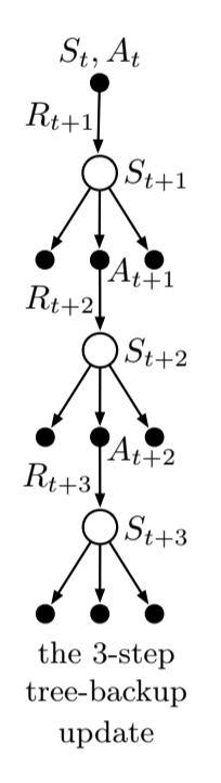
Fig 7.7. $n$-step tree

Off-policy without importance sampling: Q-learning an Expected Sarsa do it for the one-step case, and here we present a multi-step algorithm: the tree backup algorithm.

3-step tree backup diagram ->

• 3 sample states and rewards
• 2 sample actions
• list of unselected actions for each state
• We have no sample for the unselected actions, and we bootstrap with their estimated values

So far the target for the update of a node was combining the rewards along the way and the estimated values of the nodes at the bottom. Now we add to this the estimated values of the actions not selected. This is why it’s called a tree backup update: it is an update from the entire tree of estimated action values.

Each leaf node contributes to the target with a weight proportional to their probability of occurring under $\pi$.

• each first-level action $a$ contributes with a weight of $\pi(a|S_{t+1})$
• the action actually taken, $A_{t+1}$ does not contribute and its probability $\pi(A_{t+1}|S_{t+1})$ is used to weight all the second level action values.
• each second-level action $a’$ thus has a weight of $\pi(A_{t+1}|S_{t+1}) \pi(a’|S_{t+2})$

The one-step return (target) is the same as Expected Sarsa (for $t < T -1$):

$$G_{t:t+1} \doteq R_{t+1} + \gamma \sum_a \pi(a| S_{t+1}) Q_t(S_{t+1}, a) \label{eq:7.14}\tag{7.14}$$

And the two-step tree-backup return is (for $t < T -2$):

$$\begin{equation} \label{eq4} \begin{split} G_{t:t+2} & \doteq R_{t+1} + \gamma \sum_{a \neq A_{t+1}} \pi(a| S_{t+1}) Q_t(S_{t+1}, a) + \gamma \pi(A_{t+1}|S_{t+1}) \big(R_{t+2} + \gamma \sum_a \pi(a|S_{t+2}) Q_{t+1}(S_{t+2}, a)\big)\\ & = R_{t+1} + \gamma \sum_{a \neq A_{t+1}} \pi(a| S_{t+1}) Q_t(S_{t+1}, a) + \gamma \pi(A_{t+1}|S_{t+1}) G_{t+1:t+2} \end{split} \end{equation}$$

The latter form suggests the recursive form of the n-step tree backup return (for $t < T -1$):

$$G_{t:t+n} \doteq R_{t+1} + \gamma \sum_{a \neq A_{t+1}} \pi(a| S_{t+1}) Q_{t+n-1}(S_{t+1}, a) + \gamma \pi(A_{t+1}|S_{t+1}) G_{t+1:t+n} \label{eq:7.15}\tag{7.15}$$

We then use this target in the usual action-value update from n-step Sarsa:

$$Q_{t+n}(S_t, A_t) \gets Q_{t+n-1}(S_t, A_t) + \alpha \big(G_{t:t+n} - Q_{t+n-1}(S_t, A_t)\big) \label{eq:7.16}\tag{7.16}$$

Pseudocode:

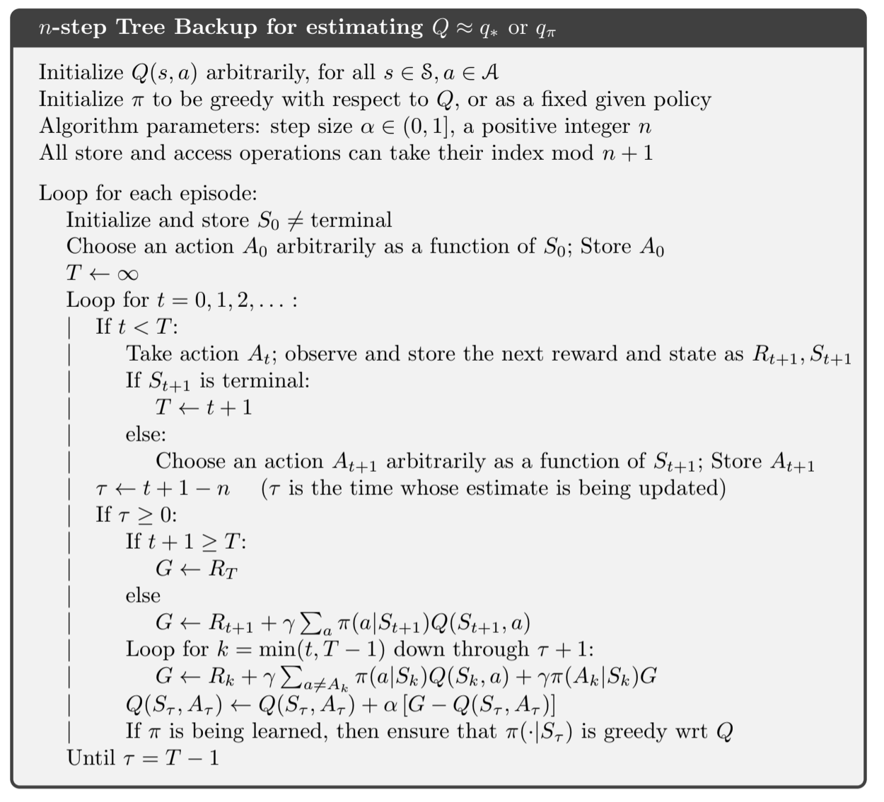
Fig 7.8. $n$-step tree backup

7.6. A Unifying algorithm: $n$-step $Q(\sigma)$

So far we have considered 3 different kinds of action-value algorithms, the 3 first of the next figure:

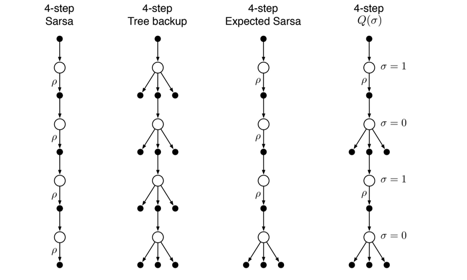
Fig 7.9. $n$-step backup diagrams. The $\rho$'s indicate half transitions on which importance sampling is required in the off-policy case.

• n-step Sarsa has all sample transitions
• the tree backup has all state-to-action transitions branched without sampling
• n-step Expected Sarsa has all sample transitions except for the last state which is fully branched with an expected value

Unification algorithm: last diagram Basic idea: decide on a step-by-step basis whether we want to sample as in Sarsa or consider the expectation over all the actions instead, as in the tree backup update.

• Let $\sigma_t \in [0, 1]$ denote the degree of sampling on step $t$, 1 being full sampling and 0 taking the expectation.
• The random variable $\sigma_t$ might be set as a function of the state, or state-action pair, at time $t$

This algorithm is called n-step $Q(\sigma)$. To develop its equations, first we need to write the tree-backup n-step return in terms of the horizon $h = t + n$ and the expected approximate value $\bar{V}$:

$$\begin{align} G_{t:h} & \doteq R_{t+1} + \gamma \sum_{a \neq A_{t+1}} \pi(a| S_{t+1}) Q_{h-1}(S_{t+1}, a) + \gamma \pi(A_{t+1}|S_{t+1}) G_{t+1:h}\\ & = R_{t+1} + \gamma \bar{V}_{h-1}(S_{t+1}) - \gamma \pi(A_{t+1} | S_{t+1}) - Q_{h-1}(S_{t+1}, A_{t+1}) + \gamma \pi(A_{t+1}|S_{t+1})G_{t+1:h}\\ & = R_{t+1} + \gamma \pi(A_{t+1} | S_{t+1}) \big( G_{t+1:h} - Q_{h-1}(S_{t+1}, A_{t+1})\big) + \gamma \bar{V}_{h-1}(S_{t+1}) \label{eq:7.17}\tag{7.17} \end{align}$$

After which this is exactly like the n-step return for Sarsa with Control Variates except with the action probability $\pi(A_{t+1}|S_{t+1})$ substituted for the importance sampling ratio $\rho_{t+1}$. For $Q(\sigma)$, we slide linearly between these two cases:

$$G_{t:h} \doteq R_{t+1} + \gamma\big(\sigma_{t+1} \rho_{t+1} + (1 - \sigma_{t+1})\pi(A_{t+1}|S_{t+1})\big)\big( G_{t+1:h} - Q_{h-1}(S_{t+1}, A_{t+1})\big)+ \gamma \bar{V}_{h-1}(S_{t+1}) \label{eq:7.18}\tag{7.18}$$

for $t < h \leq T$. The recursion ends with $G_{h:h} \doteq 0$ if $h < T$ or with $G_{T-1:T} = R_T$ if $h = T$.

Once this return is well defined, we can plug it into the usual n-step Sarsa update.

Pseudocode:

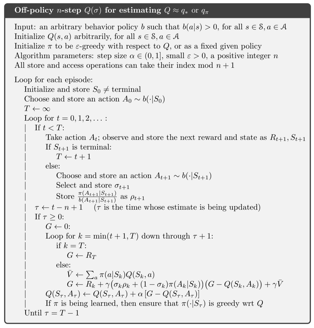
Fig 7.9. $n$-step $Q(\sigma)$

7.7. Summary

• Range of TD methods between one-step TD and Monte-Carlo methods.
• n-step methods look ahead to the next n rewards, states and actions
• all n-step methods require a delay of n steps before updating (because we need to know what happens in the next n steps) -> Eligibility traces :)
• they also involve more computation than previous methods (there is always more computation beyond the one-step methods, but it’s generally worth it since one-step is kinda limited)
• two approaches for off-policy learning have been explained:
  • one with impotance sampling is simple but has high variance
  • the other is based on tree-backup updates and is the natural extension of q-learning to multistep case with stochastic target policies